https://datascienceschool.net/view-notebook/4642b9f187784444b8f3a8309c583007/
================================================================================
* Optimization problem in math notation
* $$$x^*=\arg_x \max f(x)$$$
* Find argument solution $$$x^*$$$ which maximizes f(x)
* $$$x^*=\arg_x \min f(x)$$$
* Find argument solution $$$x^*$$$ which minimizes f(x)
* Code
* Minimization optimzation
output_data_list=function_f(input_data_list)
index_of_min_val=get_index_of_min_val(output_data_list)
arg_solution=input_data_list[index_of_min_val]
* Code
* Maximzation optimzation
output_data_list=function_f(input_data_list)
output_data_list=-output_data_list
index_of_min_val=get_index_of_min_val(output_data_list)
arg_solution=input_data_list[index_of_min_val]
* function_f: objective function, cost function, loss function, error function
================================================================================
$$$f(x)=(x-2)^2 + 2 $$$
 $$$x^{*}=\arg_x \min f(x)$$$
$$$x^{*}=2$$$
================================================================================
Rosenbrock function
$$$f(x, y) = (1 − x )^2 + 100(y − x^2)^2$$$
$$$x^{*}=\arg_x \min f(x)$$$
$$$x^{*}=2$$$
================================================================================
Rosenbrock function
$$$f(x, y) = (1 − x )^2 + 100(y − x^2)^2$$$
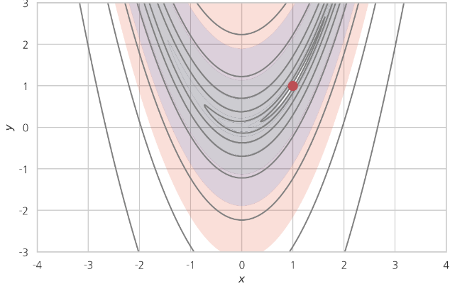 $$$x^{*},y^{*}=\arg_{x,y} \min f(x,y)$$$
$$$x^{*}=1,y^{*}=1$$$
================================================================================
* Grid search
================================================================================
* Numerical optimization:
You move x location until you find optimized y value,
as less as possible
* Tools for numerical optimzation
* Tool1: Current x location is optimal location?
* Tool2: How to find next x?
================================================================================
* Tool1: Current x location is optimal location?
- Univariate function
* $$$\dfrac{d f(x)}{dx}=0$$$
* $$$f^{'}(x)=0$$$
- Mutivariate function
* $$$\nabla f = 0$$$
* Gradient of f is 0
* $$$g=0$$$
* g: gradient of f
$$$\dfrac{\partial f(x_1,x_2,\cdots,x_N)}{\partial x_1}=0$$$
$$$\dfrac{\partial f(x_1,x_2,\cdots,x_N)}{\partial x_2}=0$$$
$$$\;\;\;\;\;\;\;\;\;\;\vdots$$$
$$$\dfrac{\partial f(x_1,x_2,\cdots,x_N)}{\partial x_N}=0$$$
* $$$g=0$$$ and $$$g' \gt 0$$$: minimum point
* $$$g=0$$$ and $$$g' \lt 0$$$: maximum point
================================================================================
* Tool2: How to find next x?
* Use SGD (Steepest Gradient Descent)
$$$x_{k+1} \\
=x_k - \alpha \times \triangledown f(x_k) \\
=x_k - \alpha \times g(x_k)$$$
* Code
alpha=learning_rate
slope_current_x=slope(current_x)
next_x=current_x-alpha*slope_current_x
If slope_current_x==0, next_x=current_x
================================================================================
$$$x_{1}$$$ -> $$$x_{2}$$$ -> $$$x_{3}$$$
$$$x^{*},y^{*}=\arg_{x,y} \min f(x,y)$$$
$$$x^{*}=1,y^{*}=1$$$
================================================================================
* Grid search
================================================================================
* Numerical optimization:
You move x location until you find optimized y value,
as less as possible
* Tools for numerical optimzation
* Tool1: Current x location is optimal location?
* Tool2: How to find next x?
================================================================================
* Tool1: Current x location is optimal location?
- Univariate function
* $$$\dfrac{d f(x)}{dx}=0$$$
* $$$f^{'}(x)=0$$$
- Mutivariate function
* $$$\nabla f = 0$$$
* Gradient of f is 0
* $$$g=0$$$
* g: gradient of f
$$$\dfrac{\partial f(x_1,x_2,\cdots,x_N)}{\partial x_1}=0$$$
$$$\dfrac{\partial f(x_1,x_2,\cdots,x_N)}{\partial x_2}=0$$$
$$$\;\;\;\;\;\;\;\;\;\;\vdots$$$
$$$\dfrac{\partial f(x_1,x_2,\cdots,x_N)}{\partial x_N}=0$$$
* $$$g=0$$$ and $$$g' \gt 0$$$: minimum point
* $$$g=0$$$ and $$$g' \lt 0$$$: maximum point
================================================================================
* Tool2: How to find next x?
* Use SGD (Steepest Gradient Descent)
$$$x_{k+1} \\
=x_k - \alpha \times \triangledown f(x_k) \\
=x_k - \alpha \times g(x_k)$$$
* Code
alpha=learning_rate
slope_current_x=slope(current_x)
next_x=current_x-alpha*slope_current_x
If slope_current_x==0, next_x=current_x
================================================================================
$$$x_{1}$$$ -> $$$x_{2}$$$ -> $$$x_{3}$$$
 ================================================================================
* Newton method which uses second order derivative
Suppose:
objective function should be second order function
Then, you can find optimal point $$$x_k$$$ by one try
Method:
Use "changed gradient vector"
changed gradient vector in its direction and length =
(inverse mat of Hessian mat) * (gradient mat)
$$${x}_{n+1} = {x}_n - [{H}f({x}_n)]^{-1} \times \nabla f({x}_n)$$$
Meaning:
1. You don't need learning rate
2. You need one order derivative (gradient vector)
3. You need second order derivative (Hessian matrix)
================================================================================
* Example of Newton method
* Second order univariate function f(x)
$$$f(x) \\
= a(x-x_0)^2 + c \\
= ax^2 -2ax_0x + x_0^2+c$$$
* $$$x^{*} = \arg_{x}\max f(x)$$$
$$$x^{*} = x_0 $$$
* Apply Newton method
$$$f'(x) = 2ax - 2ax_0$$$
$$$f''(x) = 2a$$$
$$${x}_{n+1} \\
= {x}_n - \dfrac{2ax_n - 2ax_0}{2a} \\
= x_n - (x_n - x_0) \\
= x_0$$$
================================================================================
* Limitation of Newton method
- Newton method fast converges
- But you have to find 2nd order derivative (Hessian matrix function)
- Newton method can't converges well based on shape of function
================================================================================
* Quasi-Newton method
- It doesn't use Hessian matrix function which is calculated by human
- It finds several y values at several x values around current_x
- You approximate "2nd order derivative (Hessian matrix function)"
by using above y values
- BFSG (Broyden-Fletcher-Goldfarb-Shanno) is much used
- CG (conjugated gradient) can directly calculate
"changed gradient vector (1st order derivative" without using "2nd order derivative (Hessian mat function)"
================================================================================
* Optimization by using SciPy
result=minimize(func,x0,jac=jac)
* func: objective function like $$$f(x)$$$
* x0: random initial x values
* jac: (optional) print "gradient vector (derivatives)"
* result: object of OptimizeResult
Object of OptimizeResult
x: solution x values
success: True if optimization succeeded
status: End status. 0 if optimization succeeded
message:
fun: y value at x value
jac: Value of Jacobian vector (gradient, derivative) at x
hess_inv: Value of inverse Hessian matrix at x
nfev: How many times "objective function" is called?
njev: How many times "Jacobian" is calculated?
nhev: How many times "Hessian" is calculated?
nit: How many times x is moved?
================================================================================
# Objective function
def f1(x):
return (x-2)**2+2
# c x0: random initial x value
x0=0
result=sp.optimize.minimize(f1,x0)
print(result)
# fun: 2.0
# hess_inv: array([[0.5]])
# jac: array([0.])
# message: 'Optimization terminated successfully.'
# nfev: 9
# nit: 2
# njev: 3
# status: 0
# success: True
# x: array([1.99999999])
nfev: 9 -> objective function is called 9 times
nit: 2 -> x is moved 2 times
It's because 1st order derivative (gradient vector)
and 2nd order derivative (Hessian mat function) are not given
So, SciPy had to calculate them around x values by calling objective function
================================================================================
To reduce computations, you can pass gradient vector f1p()
def f1(x):
return (x-2)**2+2
def f1p(x):
"""Derivative of f1(x)"""
return 2*(x-2)
x0=0
result = sp.optimize.minimize(f1, x0, jac=f1p)
print(result)
# fun: 2.0
# hess_inv: array([[0.5]])
# jac: array([0.])
# message: 'Optimization terminated successfully.'
# nfev: 3
# nit: 2
# njev: 3
# status: 0
# success: True
# x: array([2.])
================================================================================
* Optimization with multivariate function
def f2(x):
return (1-x[0])**2+100.0*(x[1]-x[0]**2)**2
x0=(-2,-2)
result=sp.optimize.minimize(f2,x0)
print(result)
# fun: 1.2197702024999478e-11
# hess_inv: array([[0.50957143, 1.01994476],
# [1.01994476, 2.04656074]])
# jac: array([ 9.66714798e-05, -4.64005023e-05])
# message: 'Desired error not necessarily achieved due to precision loss.'
# nfev: 496
# nit: 57
# njev: 121
# status: 2
# success: False
# x: array([0.99999746, 0.99999468])
================================================================================
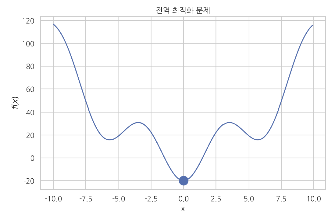
* Global optimization problem
If $$$f(x)$$$ has multiple local minima,
you can't assure numerical optimization method reaches to global minimum
Numerical optimization method depends on initial value, algorithm, parameter, etc
Reached to global minimum over local minima
================================================================================
* Newton method which uses second order derivative
Suppose:
objective function should be second order function
Then, you can find optimal point $$$x_k$$$ by one try
Method:
Use "changed gradient vector"
changed gradient vector in its direction and length =
(inverse mat of Hessian mat) * (gradient mat)
$$${x}_{n+1} = {x}_n - [{H}f({x}_n)]^{-1} \times \nabla f({x}_n)$$$
Meaning:
1. You don't need learning rate
2. You need one order derivative (gradient vector)
3. You need second order derivative (Hessian matrix)
================================================================================
* Example of Newton method
* Second order univariate function f(x)
$$$f(x) \\
= a(x-x_0)^2 + c \\
= ax^2 -2ax_0x + x_0^2+c$$$
* $$$x^{*} = \arg_{x}\max f(x)$$$
$$$x^{*} = x_0 $$$
* Apply Newton method
$$$f'(x) = 2ax - 2ax_0$$$
$$$f''(x) = 2a$$$
$$${x}_{n+1} \\
= {x}_n - \dfrac{2ax_n - 2ax_0}{2a} \\
= x_n - (x_n - x_0) \\
= x_0$$$
================================================================================
* Limitation of Newton method
- Newton method fast converges
- But you have to find 2nd order derivative (Hessian matrix function)
- Newton method can't converges well based on shape of function
================================================================================
* Quasi-Newton method
- It doesn't use Hessian matrix function which is calculated by human
- It finds several y values at several x values around current_x
- You approximate "2nd order derivative (Hessian matrix function)"
by using above y values
- BFSG (Broyden-Fletcher-Goldfarb-Shanno) is much used
- CG (conjugated gradient) can directly calculate
"changed gradient vector (1st order derivative" without using "2nd order derivative (Hessian mat function)"
================================================================================
* Optimization by using SciPy
result=minimize(func,x0,jac=jac)
* func: objective function like $$$f(x)$$$
* x0: random initial x values
* jac: (optional) print "gradient vector (derivatives)"
* result: object of OptimizeResult
Object of OptimizeResult
x: solution x values
success: True if optimization succeeded
status: End status. 0 if optimization succeeded
message:
fun: y value at x value
jac: Value of Jacobian vector (gradient, derivative) at x
hess_inv: Value of inverse Hessian matrix at x
nfev: How many times "objective function" is called?
njev: How many times "Jacobian" is calculated?
nhev: How many times "Hessian" is calculated?
nit: How many times x is moved?
================================================================================
# Objective function
def f1(x):
return (x-2)**2+2
# c x0: random initial x value
x0=0
result=sp.optimize.minimize(f1,x0)
print(result)
# fun: 2.0
# hess_inv: array([[0.5]])
# jac: array([0.])
# message: 'Optimization terminated successfully.'
# nfev: 9
# nit: 2
# njev: 3
# status: 0
# success: True
# x: array([1.99999999])
nfev: 9 -> objective function is called 9 times
nit: 2 -> x is moved 2 times
It's because 1st order derivative (gradient vector)
and 2nd order derivative (Hessian mat function) are not given
So, SciPy had to calculate them around x values by calling objective function
================================================================================
To reduce computations, you can pass gradient vector f1p()
def f1(x):
return (x-2)**2+2
def f1p(x):
"""Derivative of f1(x)"""
return 2*(x-2)
x0=0
result = sp.optimize.minimize(f1, x0, jac=f1p)
print(result)
# fun: 2.0
# hess_inv: array([[0.5]])
# jac: array([0.])
# message: 'Optimization terminated successfully.'
# nfev: 3
# nit: 2
# njev: 3
# status: 0
# success: True
# x: array([2.])
================================================================================
* Optimization with multivariate function
def f2(x):
return (1-x[0])**2+100.0*(x[1]-x[0]**2)**2
x0=(-2,-2)
result=sp.optimize.minimize(f2,x0)
print(result)
# fun: 1.2197702024999478e-11
# hess_inv: array([[0.50957143, 1.01994476],
# [1.01994476, 2.04656074]])
# jac: array([ 9.66714798e-05, -4.64005023e-05])
# message: 'Desired error not necessarily achieved due to precision loss.'
# nfev: 496
# nit: 57
# njev: 121
# status: 2
# success: False
# x: array([0.99999746, 0.99999468])
================================================================================
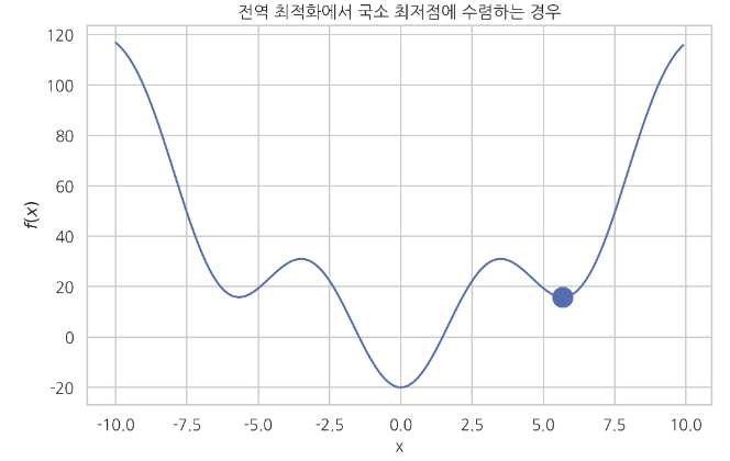
* Global optimization problem
If $$$f(x)$$$ has multiple local minima,
you can't assure numerical optimization method reaches to global minimum
Numerical optimization method depends on initial value, algorithm, parameter, etc
Reached to global minimum over local minima
 Fell into local minium
 ================================================================================
* Convex problem
* Optimzation problem
* Constraint: x range should satisfy 2nd order derivative $$$\ge$$$ 0
$$$\dfrac{\partial^2 f}{\partial x^2} \geq 0 $$$
* Constraint on multivariate function:
$$$x^THx \geq 0 \;\;\text{for all } x$$$
* Hessian function should satisfy "positive semidefinite" in given region
* It's mathematically proved that convex problem has unique minimum point
================================================================================
* Convex problem
* Optimzation problem
* Constraint: x range should satisfy 2nd order derivative $$$\ge$$$ 0
$$$\dfrac{\partial^2 f}{\partial x^2} \geq 0 $$$
* Constraint on multivariate function:
$$$x^THx \geq 0 \;\;\text{for all } x$$$
* Hessian function should satisfy "positive semidefinite" in given region
* It's mathematically proved that convex problem has unique minimum point