https://datascienceschool.net/view-notebook/87b67dafd7544e3380af278ff4f22d77/
================================================================================
9.1 모수 추정
모수 추정
데이터 분석의 첫번째 가정은 "분석하고자 하는 데이터가 어떤 확률변수로부터 실현(realized)된 표본이다"라는 가정이다.
Assumption of data analysis:
data_you_want_to_analyze=realize_event_by_random_variable(event)
이 말은 우리가 정말 관심이 있는 것이 지금 손에 가지고 있는 데이터 즉, 하나의 실현체(reailization)에 불과한 표본이 아니라 그 뒤에서 이 데이터를 만들어 내고 있는 확률변수의 분포라는 뜻이다.
Intensity of your interest:
Distribution of random_variable > data_you_want_to_analyze
확률론적인 관점에서 볼 때 데이터는 이 확률변수의 분포를 알아내기 위한 일련의 참고 자료일 뿐이다.
Within probabilisitic_perspective:
inferenced_distribution=inference_distribution_of_random_variable(data)
@@ 따라서 우리는 데이터 즉 표본으로부터 확률변수의 분포를 알아내야 한다.
그런데 확률변수의 분포가 우리가 지금까지 배운 베르누이 분포, 이항 분포, 가우시안 정규 분포 등의 기본 분포 중 하나라면 확률 분포를 알아내는 일은 다음처럼 2개의 작업으로 나뉘어진다.
확률변수가 어떤 확률분포를 따르는지 알아낸다.
확률변수(확률분포)의 모수의 값을 구한다.
distributions_list=[bernoulli,binomial,gaussian_normal,other_basic_distributions]
If distributions_you_want_to_know is in distributions_list:
# 2 steps to know distribution from data
inspected_distribution=inspect_data_to_know_kind_of_distribution(data)
inferenced_parameter_values=inference_parameter_of_the_found_distribution(data,inspected_distribution)
확률변수가 어떤 확률분포를 따르는가는 데이터가 생성되는 윈리를 알거나 다음과 같은 데이터의 여러가지 특성을 알면 추측할 수 있다.
데이터는 0 또는 1 뿐이다.
(베르누이 확률변수)
데이터는 카테고리 값이어야 한다.
(카테고리 확률변수)
데이터는 0과 1사이의 실수 값이어야 한다.
(베타 분포 확률변수)
데이터는 항상 0또는 양수이어야 한다.
(감마 분포 확률변수 또는 F-분포 확률변수)
정규 분포와 스튜던트-t 분포와 같이 구분하기 힘든 경우도 있는데 이 경우에는 뒤에서 설명할 정규성 검정(normality test)을 사용한다.
Task: find distribution kind:
if data is 0 or 1:
distribution=bernoulli_distribution
elif data is categorical values:
distribution=category_distribution
elif data is 0<=float<=1:
distribution=beta_distribution
elif data is 0 or positive_vallue:
distribution=gamma_distribution or F_distribution
elif data follows student_t_dist and gaussian_normal_dist:
ret=normality_test(data)
if ret==0:
distribution=student_t_dist
elif ret==1:
distribution=gaussian_normal_dist
두번째 작업 즉, 모수의 값으로 가장 가능성이 높은 하나의 숫자를 찾아내는 작업을 모수 추정(parameter estimation)이라고 한다.
estimated_parameter=parameter_estimation(data,found_distribution)
estimated_parameter has highest likelihood for parameter
================================================================================
모수 추정 방법론
모수 추정 방법에는 다음과 같은 방법들이 있다.
- 모멘트 방법(method of moment)
- 최대 가능도 추정(maximum likelihood estimation)
- 베이지안 추정(Bayesian estimation)
parameter_estimation_methods=[
method_of_moment,maximum_likelihood_estimation,Bayesian_estimation]
================================================================================
모멘트 방법
@@ 우선 가장 간단한 방법인 모멘트 방법부터 알아보자.
모멘트 방법(MM: Method of Moment)은 표본자료에 대한 표본 모멘트가 확률 분포의 이론적인 모멘트와 같다고 가정하고 모수를 구하는 방법이다.
Assumption:
moment of sample data == moment of probability distribution
1st moment (mean)
$$$\mu = \text{E}[X] \triangleq \bar{x} = \dfrac{1}{N} \sum_{i=1}^N x_i $$$
$$$N$$$: number of data
$$$x_i$$$: sample data
$$$\mu$$$: inferenced mean parameter (by using sample data) of probability distribution
2차 모멘트(분산)의 경우에는 다음과 같다.
2nd moment (variance)
$$$ \sigma^2 = \text{E}[(X-\mu)^2] \triangleq \bar{s}^2 = \dfrac{1}{N-1} \sum_{i=1}^N (x_i - \bar{x})^2 $$$
$$$\sigma^2$$$: inferenced variance parameter (by using sample data) of probability distribution
================================================================================
모멘트 방법을 사용한 베르누이 분포의 모수 추정
모멘트 방법으로 베르누이 확률변수의 모수 $$$\mu$$$ 를 구하면 다음과 같다.
Inference parameter $$$\mu$$$ of Bernoulli distribution by using moment method
이 식에서 $$$N_1$$$ 은 1의 갯수이다.
$$$N_1$$$: number of data "1"
$$$ \text{E}[X] = \mu \triangleq \bar{x} = \dfrac{1}{N} \sum_{i=1}^N x_i = \dfrac{N_1}{N} $$$
param_mu=estimate_parameter(sample_data)
================================================================================
모멘트 방법을 사용한 정규 분포의 모수 추정
모멘트 방법으로 정규 분포의 모수 $$$\mu$$$, $$$\sigma^2$$$ 를 구하면 다음과 같다.
mean_param,variance_param=estimate_parameters_using_moment_method(data)
$$$ \text{E}[X] = \mu \triangleq \bar{x} = \dfrac{1}{N} \sum_{i=1}^N x_i $$$
mean_param=estimate_mean_param(data,num_of_data)
$$$ \text{E}[(X-\mu)^2] = \sigma^2 \triangleq s^2 = \dfrac{1}{N-1} \sum_{i=1}^N (x_i - \bar{x})^2 $$$
variance_param=estimate_variance_param(data,num_of_data)
정규분포는 모수가 아예 모멘트로 정의되어 있기 때문에 모멘트 방법을 사용하면 아주 쉽게 모수를 추정할 수 있다.
Parameters of normal distribution are defined by "moment"
================================================================================
모멘트 방법을 사용한 베타 분포의 모수 추정
모멘트 방법으로 베타 분포의 모수 a, b 를 구하면 다음과 같다.
param_a,param_b=estimate_param_using_moment_method(data)
이 경우에는 모수와 모멘트 간의 관계를 이용하여 비선형 연립 방정식을 풀어야 한다.
You should solve following non-linear simultaneous equation
$$$ \text{E}[X] = \dfrac{a}{a+b} \triangleq \bar{x} $$$
$$$ \text{E}[(X-\mu)^2] = \dfrac{ab}{(a+b)^2(a+b+1)} \triangleq s^2 $$$
이 비선형 연립방정식을 풀어 해를 구하면 다음과 같다.
You can get the solution
$$$ a = \bar{x} \left( \frac{\bar{x} (1 - \bar{x})}{s^2} - 1 \right) $$$
$$$ b = (1 - \bar{x}) \left( \frac{\bar{x} (1 - \bar{x})}{s^2} - 1 \right) $$$
================================================================================
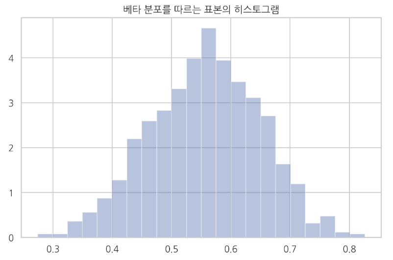
예를 들어 a=15,b=12 인 베타 분포의 데이터 100개로부터 모멘트 방법으로 모수를 추정하면 다음과 같다.
Create following beta distribution
- Parameters: a=15,b=15
- 100 data which follows beta distribution
np.random.seed(0)
x = sp.stats.beta(15, 12).rvs(1000)
sns.distplot(x, kde=False, norm_hist=True)
plt.title("Histogram plot which is plotted by using 1000 number of sample data which follows beta distribution")
plt.show()
 ================================================================================
- Estimate parameters a and b of beta distribution
- by using 1000 number of sample data which follows beta distribution
def estimate_beta(x):
x_bar = x.mean()
s2 = x.var()
a = x_bar * (x_bar * (1 - x_bar) / s2 - 1)
b = (1 - x_bar) * (x_bar * (1 - x_bar) / s2 - 1)
return a, b
params = estimate_beta(x)
print(params)
# (15.455080715555846, 12.292335248133712)
================================================================================
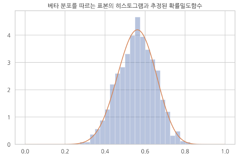
Estimated beta distribution
xx = np.linspace(0, 1, 1000)
sns.distplot(x, kde=False, norm_hist=True)
plt.plot(xx, sp.stats.beta(params[0], params[1]).pdf(xx))
plt.title("Histogram: actual data, Curve line: estimated PDF of beta distribution")
plt.show()
================================================================================
- Estimate parameters a and b of beta distribution
- by using 1000 number of sample data which follows beta distribution
def estimate_beta(x):
x_bar = x.mean()
s2 = x.var()
a = x_bar * (x_bar * (1 - x_bar) / s2 - 1)
b = (1 - x_bar) * (x_bar * (1 - x_bar) / s2 - 1)
return a, b
params = estimate_beta(x)
print(params)
# (15.455080715555846, 12.292335248133712)
================================================================================
Estimated beta distribution
xx = np.linspace(0, 1, 1000)
sns.distplot(x, kde=False, norm_hist=True)
plt.plot(xx, sp.stats.beta(params[0], params[1]).pdf(xx))
plt.title("Histogram: actual data, Curve line: estimated PDF of beta distribution")
plt.show()