https://datascienceschool.net/view-notebook/58269d7f52bd49879965cdc4721da42d/
================================================================================
* regression analysis
* regression analysis quantitatively finds the relationship
between D-dim vector independent variable x and scalar dependent variable y
* regression analysis: deterministic model, probabilistic model
================================================================================
* deterministic model
* deterministic model should find f(x) satisfying following
$$$\hat{y} = f(x) \approx y$$$
* If $$$f(x)$$$ is following-like linear function, it's called linear regression
$$$\hat{y} \\
= w_0 + w_1 x_1 + w_2 x_2 + \cdots + w_D x_D \\
= w_0 + w^Tx$$$
* $$$w_0,\cdots, w_D$$$: parameter of linear regression model, coefficient of $$$f(x)$$$
================================================================================
* If linear regression model has "constant term",
you can insert "constant term" into feature vector
* It is called "bias augmentation"
$$$x_i =
\begin{bmatrix}
x_{i1} \\ x_{i2} \\ \vdots \\ x_{iD}
\end{bmatrix}$$$
Insert constant term 1
$$$x_{i,a} =
\begin{bmatrix}
1 \\ x_{i1} \\ x_{i2} \\ \vdots \\ x_{iD}
\end{bmatrix}$$$
================================================================================
* Use "bias augmentation" on multiple feature vectors
$$$X =
\begin{bmatrix}
x_{11} & x_{12} & \cdots & x_{1D} \\
x_{21} & x_{22} & \cdots & x_{2D} \\
\vdots & \vdots & \vdots & \vdots \\
x_{N1} & x_{N2} & \cdots & x_{ND} \\
\end{bmatrix}$$$
Insert constant term into all feature vectors as bias
$$$X_a =
\begin{bmatrix}
1 & x_{11} & x_{12} & \cdots & x_{1D} \\
1 & x_{21} & x_{22} & \cdots & x_{2D} \\
\vdots & \vdots & \vdots & \vdots & \vdots \\
1 & x_{N1} & x_{N2} & \cdots & x_{ND} \\
\end{bmatrix}$$$
================================================================================
* Linear regression function f(x) which has constant term will look like
$$$f(x) = w_0 + w_1 x_1 + w_2 x_2 + \cdots + w_D x_D$$$
* It can be expressed by matrix multiplication
$$$= \begin{bmatrix}
1 & x_1 & x_2 & \cdots & x_D
\end{bmatrix}
\begin{bmatrix}
w_0 \\ w_1 \\ w_2 \\ \vdots \\ w_D
\end{bmatrix}$$$
* You can simplify above matrix multiplication
$$$= x_a^T w_a = w_a^T x_a$$$
================================================================================
* Code
# ================================================================================
from sklearn.datasets import make_regression
import numpy as np
import statsmodels.api as sm
# ================================================================================
X0,y,coef=make_regression(
n_samples=100,n_features=2,bias=100,noise=10,coef=True,random_state=1)
# c ori_feat_vecs: original feature vectors
ori_feat_vecs=X0[:5]
# print("ori_feat_vecs",ori_feat_vecs)
# [[ 0.0465673 0.80186103]
# [-2.02220122 0.31563495]
# [-0.38405435 -0.3224172 ]
# [-1.31228341 0.35054598]
# [-0.88762896 -0.19183555]]
# ================================================================================
# Create constant terms
one_vecs=np.ones((X0.shape[0],1))
# print("one_vecs",one_vecs)
# [[1.]
# [1.]
# ================================================================================
# Perform "bias augmentation" (inserting constant term into feature vectors)
stacked_arr=np.hstack((one_vecs,X0))
# print("stacked_arr",stacked_arr)
# [[ 1. 0.0465673 0.80186103]
# [ 1. -2.02220122 0.31563495]
# [ 1. -0.38405435 -0.3224172 ]
# ================================================================================
# You can perform "bias augmentation" by using statsmodels.api.add_constant()
X = sm.add_constant(X0)
# print("X",X)
# [[ 1. 0.0465673 0.80186103]
# [ 1. -2.02220122 0.31563495]
# [ 1. -0.38405435 -0.3224172 ]
================================================================================
* Ordinary Least Squares (OLS)
* Basic method for deterministic linear regression
* It finds parameters which minimize "Residual Sum of Squares"
by using matrix differentiation
* Linear regression model: $$$\hat{y}=X\omega$$$
* $$$X$$$: feature vectors
* $$$\omega$$$: trainable parameters
* Residual vector e:
$$$e \\
=y-\hat{y} \\
=y-X\omega$$$
* Residual Sum of Squares
$$$RSS \\
= e^Te \\
= (y-X\omega)^T(y-X\omega) \\
= y^Ty-2y^TX\omega+\omega^TX^TX\omega$$$
================================================================================
* You should find minimum value from RSS
So, you perform differentiation
$$$\dfrac{d \text{RSS}}{d w} = -2 X^T y + 2 X^TX w$$$
* You put 0 to find minimum value
$$$\dfrac{d \text{RSS}}{d w} = 0$$$
* $$$X^TX w^{\ast} = X^T y$$$
================================================================================
* If inverse matrix of $$$X^TX$$$ exist, you can find optimal parameter $$$\omega$$$
$$$w^{\ast} = (X^TX)^{-1} X^T y$$$
================================================================================
* Normal equation
* Equation which has 0 in its gradient
$$$\dfrac{d \text{RSS}}{d w} = 0$$$
$$$X^TX w^{\ast} = X^T y$$$
$$$X^T y - X^TX w = 0$$$
================================================================================
* Code
* Linear regression analysis by using NumPy
from sklearn.datasets import make_regression
bias=100
X0,y,coef=make_regression(
n_samples=100,n_features=1,bias=bias,noise=10,coef=True,random_state=1)
# print("X0",X0)
# [[-0.61175641]
# [-0.24937038]
# print("y",y)
# y [ 47.5431146 84.60560134
# print("coef",coef)
# 80.71051956187792
X=sm.add_constant(X0)
# print("X",X)
# [[ 1. -0.61175641]
# [ 1. -0.24937038]
y=y.reshape(len(y),1)
# print("y",y)
# [[ 47.5431146 ]
# [ 84.60560134]
# ================================================================================
# Relationship between x and y in linear regression model
# $$$y = 100 + 80.7105 x + \epsilon$$$
# $$$y=bias + Wx + \epsilon$$$
# # ================================================================================
# * Get bias (100) and weight (80) manually
# $$$X^T\cdot X$$$
sqr_mat=np.dot(X.T,X)
# print("sqr_mat",sqr_mat)
# [[100. 6.05828521]
# [ 6.05828521 78.71718049]]
# (X^TX)^{-1}
inv_of_sqr_mat=np.linalg.inv(sqr_mat)
# print("inv_of_sqr_mat",inv_of_sqr_mat)
# [[ 0.01004684 -0.00077323]
# [-0.00077323 0.01276322]]
# $$$(X^TX)^{-1}\cdot X^T$$$
sqr_mat=np.dot(inv_of_sqr_mat,X.T)
# print("sqr_mat",sqr_mat)
# [[ 0.01051987 0.01023967 0.00966911 0.00945763 0.00887167 0.0097549
# 0.00965023 0.01056587 0.01112666 0.00980279 0.01053939 0.01035363
# print("sqr_mat",sqr_mat.shape)
# (2, 100)
# $$$((X^TX)^{-1}\cdot X^T)\cdot y$$$
X_mul_y=np.dot(sqr_mat,y)
# print("X_mul_y",X_mul_y)
# [[102.02701439]
# [ 81.59750943]]
# \hat{y} = 102.02701439 + 81.59750943x
# ================================================================================
# \hat{y}=WX+b
# Find W and b
sol=np.linalg.lstsq(X,y)
# print("sol",sol)
# (array([[102.02701439],
# [ 81.59750943]]),
# array([8314.18911692]),
# 2,
# array([10.07986548, 8.78142884]))
# ================================================================================
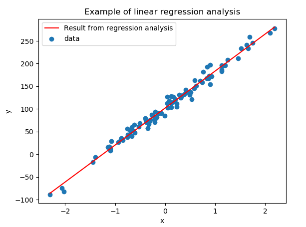
x_new = np.linspace(np.min(X0), np.max(X0), 100)
X_new = sm.add_constant(x_new) # 상수항 결합
# y_new = np.dot(X_new, X_mul_y)
y_new = np.dot(X_new, sol[0])
plt.scatter(X0, y, label="data")
plt.plot(x_new, y_new, 'r-', label="Result from regression analysis")
plt.xlabel("x")
plt.ylabel("y")
plt.title("Example of linear regression analysis")
plt.legend()
plt.show()
 # ================================================================================
# * Linear regression analysis by using scikit-learn
# 1. Create object of LinearRegreeson
# model=LinearRegreeson(fit_intercept=True)
# * fit_intercept
# True: model contains constant term
# False: model contains no constant term
# 2. Perform "inference model", "bias augmentation" by using fit()
# modle=model.fit(X,y)
# Return:
# * LinearRegreeson itself but it contains data
# * coef_: inferenced trainable weight vectors
# * intercept_: inferenced constant terms
# 3. Make a prediction by using predict()
# y_pred=model.predict(x_new)
# ================================================================================
# * Code
# * Linear regression analysis by using scikit-learn
from sklearn.datasets import load_boston
from sklearn.linear_model import LinearRegression
boston=load_boston()
X=boston.data
# print("X",X)
# [[6.3200e-03 1.8000e+01 2.3100e+00 ... 1.5300e+01 3.9690e+02 4.9800e+00]
# [2.7310e-02 0.0000e+00 7.0700e+00 ... 1.7800e+01 3.9690e+02 9.1400e+00]
y=boston.target
# print("y",y)
# [24. 21.6 34.7 33.4 36.2 28.7 22.9 27.1 16.5 18.9 15. 18.9 21.7 20.4
# 18.2 19.9 23.1 17.5 20.2 18.2 13.6 19.6 15.2 14.5 15.6 13.9 16.6 14.8
model_boston=LinearRegression().fit(X,y)
# print("model_boston.coef_",model_boston.coef_)
# [-1.08011358e-01 4.64204584e-02 2.05586264e-02 2.68673382e+00
# -1.77666112e+01 3.80986521e+00 6.92224640e-04 -1.47556685e+00
# Meaning:
# If room (RM) increases by 1, predicted price y increases (3810 dollars)
# print("boston",boston.feature_names)
# ['CRIM' 'ZN' 'INDUS' 'CHAS' 'NOX' 'RM' 'AGE' 'DIS' 'RAD' 'TAX' 'PTRATIO' 'B' 'LSTAT']
# print("model_boston.intercept_",model_boston.intercept_)
# 36.459488385090054
# ================================================================================
X_data=boston.data
y_true_price=boston.target
y_pred_price=model_boston.predict(X_data)
# plt.scatter(y_true_price,y_pred_price)
# plt.xlabel(u"True price")
# plt.ylabel(u"Pred price")
# plt.title("Relationship between true price and predicted price")
# plt.show()
# ================================================================================
# * Linear regression analysis by using scikit-learn
# 1. Create object of LinearRegreeson
# model=LinearRegreeson(fit_intercept=True)
# * fit_intercept
# True: model contains constant term
# False: model contains no constant term
# 2. Perform "inference model", "bias augmentation" by using fit()
# modle=model.fit(X,y)
# Return:
# * LinearRegreeson itself but it contains data
# * coef_: inferenced trainable weight vectors
# * intercept_: inferenced constant terms
# 3. Make a prediction by using predict()
# y_pred=model.predict(x_new)
# ================================================================================
# * Code
# * Linear regression analysis by using scikit-learn
from sklearn.datasets import load_boston
from sklearn.linear_model import LinearRegression
boston=load_boston()
X=boston.data
# print("X",X)
# [[6.3200e-03 1.8000e+01 2.3100e+00 ... 1.5300e+01 3.9690e+02 4.9800e+00]
# [2.7310e-02 0.0000e+00 7.0700e+00 ... 1.7800e+01 3.9690e+02 9.1400e+00]
y=boston.target
# print("y",y)
# [24. 21.6 34.7 33.4 36.2 28.7 22.9 27.1 16.5 18.9 15. 18.9 21.7 20.4
# 18.2 19.9 23.1 17.5 20.2 18.2 13.6 19.6 15.2 14.5 15.6 13.9 16.6 14.8
model_boston=LinearRegression().fit(X,y)
# print("model_boston.coef_",model_boston.coef_)
# [-1.08011358e-01 4.64204584e-02 2.05586264e-02 2.68673382e+00
# -1.77666112e+01 3.80986521e+00 6.92224640e-04 -1.47556685e+00
# Meaning:
# If room (RM) increases by 1, predicted price y increases (3810 dollars)
# print("boston",boston.feature_names)
# ['CRIM' 'ZN' 'INDUS' 'CHAS' 'NOX' 'RM' 'AGE' 'DIS' 'RAD' 'TAX' 'PTRATIO' 'B' 'LSTAT']
# print("model_boston.intercept_",model_boston.intercept_)
# 36.459488385090054
# ================================================================================
X_data=boston.data
y_true_price=boston.target
y_pred_price=model_boston.predict(X_data)
# plt.scatter(y_true_price,y_pred_price)
# plt.xlabel(u"True price")
# plt.ylabel(u"Pred price")
# plt.title("Relationship between true price and predicted price")
# plt.show()
 # ================================================================================
# * Linear regression analysis by using statsmodel
# 1. Create OLS (Ordinary Least Squares)
# If you need, use add_constant() to add constant term
# model=OLS(y,X)
# 2. Inference model
# result=model.fit()
# result: RegressionResults object
# 3. Create report and prediction
# print("result.summary()",result.summary())
# y_pred=result.predict(x_new)
# If you performed "bias augmentation",
# you also should perform "bias augmentation" to x_new
# ================================================================================
# * Code
X_data=boston.data
X_data_feat_names=boston.feature_names
X_wo_const_term=pd.DataFrame(X_data,columns=X_data_feat_names)
X_w_const_term=sm.add_constant(X_wo_const_term)
y_data=boston.target
y_data=pd.DataFrame(y_data,columns=["MEDV"])
lin_reg_model=sm.OLS(y_data,X_w_const_term)
trained_lin_reg_model=lin_reg_model.fit()
# print("trained_lin_reg_model.summary()",trained_lin_reg_model.summary())
# OLS Regression Results
# ==============================================================================
# Dep. Variable: MEDV R-squared: 0.741
# Model: OLS Adj. R-squared: 0.734
# Method: Least Squares F-statistic: 108.1
# Date: 화, 07 5월 2019 Prob (F-statistic): 6.72e-135
# Time: 11:31:01 Log-Likelihood: -1498.8
# No. Observations: 506 AIC: 3026.
# Df Residuals: 492 BIC: 3085.
# Df Model: 13
# Covariance Type: nonrobust
# ==============================================================================
# coef std err t P>|t| [0.025 0.975]
# ------------------------------------------------------------------------------
# const 36.4595 5.103 7.144 0.000 26.432 46.487
# CRIM -0.1080 0.033 -3.287 0.001 -0.173 -0.043
# ZN 0.0464 0.014 3.382 0.001 0.019 0.073
# INDUS 0.0206 0.061 0.334 0.738 -0.100 0.141
# CHAS 2.6867 0.862 3.118 0.002 0.994 4.380
# NOX -17.7666 3.820 -4.651 0.000 -25.272 -10.262
# RM 3.8099 0.418 9.116 0.000 2.989 4.631
# AGE 0.0007 0.013 0.052 0.958 -0.025 0.027
# DIS -1.4756 0.199 -7.398 0.000 -1.867 -1.084
# RAD 0.3060 0.066 4.613 0.000 0.176 0.436
# TAX -0.0123 0.004 -3.280 0.001 -0.020 -0.005
# PTRATIO -0.9527 0.131 -7.283 0.000 -1.210 -0.696
# B 0.0093 0.003 3.467 0.001 0.004 0.015
# LSTAT -0.5248 0.051 -10.347 0.000 -0.624 -0.425
# ==============================================================================
# Omnibus: 178.041 Durbin-Watson: 1.078
# Prob(Omnibus): 0.000 Jarque-Bera (JB): 783.126
# Skew: 1.521 Prob(JB): 8.84e-171
# Kurtosis: 8.281 Cond. No. 1.51e+04
# ==============================================================================
# Warnings:
# [1] Standard Errors assume that the covariance matrix of the errors is correctly specified.
# [2] The condition number is large, 1.51e+04. This might indicate that there are
# strong multicollinearity or other numerical problems.
# ================================================================================
# print("X_wo_const_term",X_wo_const_term.shape)
# (506, 13)
# print("X_wo_const_term",X_wo_const_term)
# CRIM ZN INDUS CHAS ... TAX PTRATIO B LSTAT
# 0 0.00632 18.0 2.31 0.0 ... 296.0 15.3 396.90 4.98
# 1 0.02731 0.0 7.07 0.0 ... 242.0 17.8 396.90 9.14
mean_of_X_wo_const_term=X_wo_const_term.mean().values
# print("mean_of_X_wo_const_term",mean_of_X_wo_const_term.shape)
# (13,)
# print("mean_of_X_wo_const_term",mean_of_X_wo_const_term)
# [3.61352356e+00 1.13636364e+01 1.11367787e+01 6.91699605e-02
# 5.54695059e-01 6.28463439e+00 6.85749012e+01 3.79504269e+00
# 9.54940711e+00 4.08237154e+02 1.84555336e+01 3.56674032e+02
# 1.26530632e+01]
================================================================================
# ================================================================================
# * Linear regression analysis by using statsmodel
# 1. Create OLS (Ordinary Least Squares)
# If you need, use add_constant() to add constant term
# model=OLS(y,X)
# 2. Inference model
# result=model.fit()
# result: RegressionResults object
# 3. Create report and prediction
# print("result.summary()",result.summary())
# y_pred=result.predict(x_new)
# If you performed "bias augmentation",
# you also should perform "bias augmentation" to x_new
# ================================================================================
# * Code
X_data=boston.data
X_data_feat_names=boston.feature_names
X_wo_const_term=pd.DataFrame(X_data,columns=X_data_feat_names)
X_w_const_term=sm.add_constant(X_wo_const_term)
y_data=boston.target
y_data=pd.DataFrame(y_data,columns=["MEDV"])
lin_reg_model=sm.OLS(y_data,X_w_const_term)
trained_lin_reg_model=lin_reg_model.fit()
# print("trained_lin_reg_model.summary()",trained_lin_reg_model.summary())
# OLS Regression Results
# ==============================================================================
# Dep. Variable: MEDV R-squared: 0.741
# Model: OLS Adj. R-squared: 0.734
# Method: Least Squares F-statistic: 108.1
# Date: 화, 07 5월 2019 Prob (F-statistic): 6.72e-135
# Time: 11:31:01 Log-Likelihood: -1498.8
# No. Observations: 506 AIC: 3026.
# Df Residuals: 492 BIC: 3085.
# Df Model: 13
# Covariance Type: nonrobust
# ==============================================================================
# coef std err t P>|t| [0.025 0.975]
# ------------------------------------------------------------------------------
# const 36.4595 5.103 7.144 0.000 26.432 46.487
# CRIM -0.1080 0.033 -3.287 0.001 -0.173 -0.043
# ZN 0.0464 0.014 3.382 0.001 0.019 0.073
# INDUS 0.0206 0.061 0.334 0.738 -0.100 0.141
# CHAS 2.6867 0.862 3.118 0.002 0.994 4.380
# NOX -17.7666 3.820 -4.651 0.000 -25.272 -10.262
# RM 3.8099 0.418 9.116 0.000 2.989 4.631
# AGE 0.0007 0.013 0.052 0.958 -0.025 0.027
# DIS -1.4756 0.199 -7.398 0.000 -1.867 -1.084
# RAD 0.3060 0.066 4.613 0.000 0.176 0.436
# TAX -0.0123 0.004 -3.280 0.001 -0.020 -0.005
# PTRATIO -0.9527 0.131 -7.283 0.000 -1.210 -0.696
# B 0.0093 0.003 3.467 0.001 0.004 0.015
# LSTAT -0.5248 0.051 -10.347 0.000 -0.624 -0.425
# ==============================================================================
# Omnibus: 178.041 Durbin-Watson: 1.078
# Prob(Omnibus): 0.000 Jarque-Bera (JB): 783.126
# Skew: 1.521 Prob(JB): 8.84e-171
# Kurtosis: 8.281 Cond. No. 1.51e+04
# ==============================================================================
# Warnings:
# [1] Standard Errors assume that the covariance matrix of the errors is correctly specified.
# [2] The condition number is large, 1.51e+04. This might indicate that there are
# strong multicollinearity or other numerical problems.
# ================================================================================
# print("X_wo_const_term",X_wo_const_term.shape)
# (506, 13)
# print("X_wo_const_term",X_wo_const_term)
# CRIM ZN INDUS CHAS ... TAX PTRATIO B LSTAT
# 0 0.00632 18.0 2.31 0.0 ... 296.0 15.3 396.90 4.98
# 1 0.02731 0.0 7.07 0.0 ... 242.0 17.8 396.90 9.14
mean_of_X_wo_const_term=X_wo_const_term.mean().values
# print("mean_of_X_wo_const_term",mean_of_X_wo_const_term.shape)
# (13,)
# print("mean_of_X_wo_const_term",mean_of_X_wo_const_term)
# [3.61352356e+00 1.13636364e+01 1.11367787e+01 6.91699605e-02
# 5.54695059e-01 6.28463439e+00 6.85749012e+01 3.79504269e+00
# 9.54940711e+00 4.08237154e+02 1.84555336e+01 3.56674032e+02
# 1.26530632e+01]
================================================================================