================================================================================
* $$$x_1,x_2,\cdots,x_D$$$: D number of independent variables
* Linear regression model: $$$\hat{y} \sim x_1+x_2+\cdots+x_D$$$
* Suppose $$$x_1$$$ independent variable is range type variable
* $$$x_1$$$ can have "man" or "woman"
* You can use dummy variable d
* x="man" to d=(1,0)
* x="woman" to d=(0,1)
* Model:
$$$\hat{y}=[\omega_{d1}d_1 + \omega_{d2}d_2] + \omega_2x_2+\cdots+\omega_Dx_D$$$
================================================================================
* Full rank dummy variable model
x="A blood type" -> d=(1,0,0,0)
x="AB blood type" -> d=(1,1,0,0)
x="B blood type" -> d=(1,0,1,0)
x="O blood type" -> d=(1,0,0,1)
* Reduced rank dummy variable model which uses one-hot-encoding
x="A blood type" -> d=(1,0,0,0)
x="AB blood type" -> d=(0,1,0,0)
x="B blood type" -> d=(0,0,1,0)
x="O blood type" -> d=(0,0,0,1)
================================================================================
# conda activate py36gputorch100 && \
# cd /mnt/1T-5e7/mycodehtml/ML_theory/DHKim/003_Regression_ananalysis_and_Timeseries_analysis/002_Basic_of_linear_regression/02.03_Range_datatype_independent_variable && \
# rm e.l && python main.py \
# 2>&1 | tee -a e.l && code e.l
# ================================================================================
from sklearn.datasets import make_regression
import numpy as np
import pandas as pd
import statsmodels.api as sm
import matplotlib.pyplot as plt
from patsy import *
import datetime
from calendar import isleap
import scipy as sp
import statsmodels.formula.api as smf
import statsmodels.stats.api as sms
import sklearn as sk
from sklearn.datasets import load_boston
import matplotlib as mpl
from mpl_toolkits.mplot3d import Axes3D
import seaborn as sns
# ================================================================================
# * Linear regression on a model which has range type independet variable
# * independent variable: monthh
# * dependent variable: temperature
# ================================================================================
df_nottem=sm.datasets.get_rdataset("nottem").data
# print("df_nottem",df_nottem)
# time value
# 0 1920.000000 40.6
# 1 1920.083333 40.8
# ================================================================================
def convert_partial_year(number):
year=int(number)
d=datetime.timedelta(days=(number-year)*(365+isleap(year)))
day_one=datetime.datetime(year,1,1)
date=d+day_one
return date
# ================================================================================
time_col_data=df_nottem[["time"]]
# print("time_col_data",time_col_data)
# time
# 0 1920.000000
# 1 1920.083333
df_nottem["date0"]=time_col_data.applymap(convert_partial_year)
# ================================================================================
date0_col_data=df_nottem["date0"]
# print("date0_col_data",date0_col_data)
# 0 1920-01-01 00:00:00.000000
# 1 1920-01-31 11:59:59.999897
dt_idx_of_date0_col_data=pd.DatetimeIndex(date0_col_data)
# print("dt_idx_of_date0_col_data",dt_idx_of_date0_col_data)
# DatetimeIndex([ '1920-01-01 00:00:00', '1920-01-31 11:59:59.999897',
# '1920-03-02 00:00:00.000103', '1920-04-01 12:00:00',
# '1920-05-01 23:59:59.999897', '1920-06-01 12:00:00.000103',
rounded=dt_idx_of_date0_col_data.round('60min')
# print("rounded",rounded)
# DatetimeIndex(['1920-01-01 00:00:00', '1920-01-31 12:00:00',
# '1920-03-02 00:00:00', '1920-04-01 12:00:00',
# '1920-05-02 00:00:00', '1920-06-01 12:00:00',
sec_of_one_day=datetime.timedelta(seconds=3600*24)
# print("sec_of_one_day",sec_of_one_day)
# 1 day, 0:00:00
final_date_data=rounded+sec_of_one_day
# print("final_date_data",final_date_data)
# DatetimeIndex(['1920-01-02 00:00:00', '1920-02-01 12:00:00',
# '1920-03-03 00:00:00', '1920-04-02 12:00:00',
# '1920-05-03 00:00:00', '1920-06-02 12:00:00',
df_nottem["date"]=final_date_data
# ================================================================================
df_nottem["month"] = df_nottem["date"].dt.strftime("%m").astype('category')
del df_nottem["date0"], df_nottem["date"]
# ================================================================================
# print("df_nottem.tail()",df_nottem.tail())
# time value month
# 235 1939.583333 61.8 08
# 236 1939.666667 58.2 09
# ================================================================================
df_nottem.boxplot("value", "month")
plt.show()
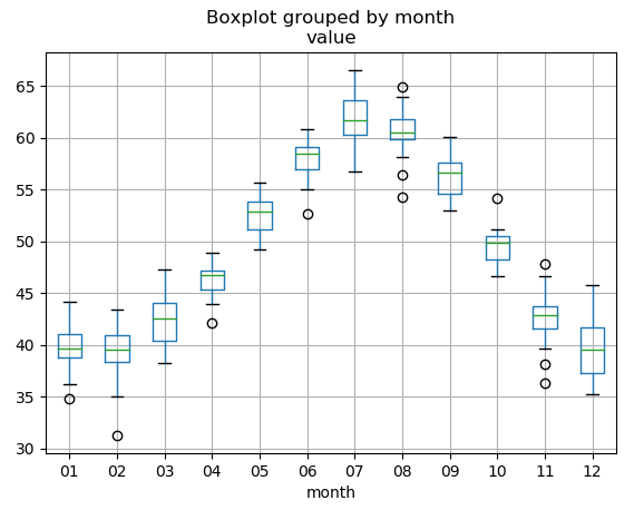 # Meaning:
# 4,6,8,11 have small difference
# Temperature is highest at 6,7,8
# Temperature is lowerest at 1,2,12
# ================================================================================
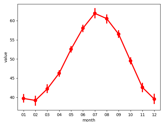
sns.stripplot(x="month", y="value", data=df_nottem, jitter=True, alpha=.3)
# plt.show()
#
# Meaning:
# 4,6,8,11 have small difference
# Temperature is highest at 6,7,8
# Temperature is lowerest at 1,2,12
# ================================================================================
sns.stripplot(x="month", y="value", data=df_nottem, jitter=True, alpha=.3)
# plt.show()
#  sns.pointplot(x="month", y="value", data=df_nottem, dodge=True, color='r')
# plt.show()
#
sns.pointplot(x="month", y="value", data=df_nottem, dodge=True, color='r')
# plt.show()
#  #
#  # ================================================================================
# Inference linear regression model
model = sm.OLS.from_formula("value ~ C(month) + 0", df_nottem)
result = model.fit()
# print(result.summary())
# OLS Regression Results
# ==============================================================================
# Dep. Variable: value R-squared: 0.930
# Model: OLS Adj. R-squared: 0.927
# Method: Least Squares F-statistic: 277.3
# Date: 화, 07 5월 2019 Prob (F-statistic): 2.96e-125
# Time: 13:14:36 Log-Likelihood: -535.82
# No. Observations: 240 AIC: 1096.
# Df Residuals: 228 BIC: 1137.
# Df Model: 11
# Covariance Type: nonrobust
# ================================================================================
# coef std err t P>|t| [0.025 0.975]
# --------------------------------------------------------------------------------
# C(month)[01] 39.6950 0.518 76.691 0.000 38.675 40.715
# C(month)[02] 39.1900 0.518 75.716 0.000 38.170 40.210
# C(month)[03] 42.1950 0.518 81.521 0.000 41.175 43.215
# C(month)[04] 46.2900 0.518 89.433 0.000 45.270 47.310
# C(month)[05] 52.5600 0.518 101.547 0.000 51.540 53.580
# C(month)[06] 58.0400 0.518 112.134 0.000 57.020 59.060
# C(month)[07] 61.9000 0.518 119.592 0.000 60.880 62.920
# C(month)[08] 60.5200 0.518 116.926 0.000 59.500 61.540
# C(month)[09] 56.4800 0.518 109.120 0.000 55.460 57.500
# C(month)[10] 49.4950 0.518 95.625 0.000 48.475 50.515
# C(month)[11] 42.5800 0.518 82.265 0.000 41.560 43.600
# C(month)[12] 39.5300 0.518 76.373 0.000 38.510 40.550
# ==============================================================================
# Omnibus: 5.430 Durbin-Watson: 1.529
# Prob(Omnibus): 0.066 Jarque-Bera (JB): 5.299
# Skew: -0.281 Prob(JB): 0.0707
# Kurtosis: 3.463 Cond. No. 1.00
# ==============================================================================
# Warnings:
# [1] Standard Errors assume that the covariance matrix of the errors is correctly specified.
# ================================================================================
# If you delete "+0" from string of formula, you will use full rank dummy variable
model = sm.OLS.from_formula("value ~ C(month)", df_nottem)
result = model.fit()
# print(result.summary())
# ================================================================================
# * Boston house price has range type data (0 or 1) on CHAS column
# * Model equation
# When CHAS=1,
# $$$y = (w_0 + w_{\text{CHAS}}) + w_{\text{CRIM}} \text{CRIM} + w_{\text{ZN}} \text{ZN} + \cdots$$$
# When CHAS=0,
# $$$y = w_0 + w_{\text{CRIM}} \text{CRIM} + w_{\text{ZN}} \text{ZN} + \cdots$$$
boston=load_boston()
X_feat_data=boston.data
X_feat_names=boston.feature_names
X_wo_constant_term=pd.DataFrame(X_feat_data,columns=X_feat_names)
X_w_constant_term=sm.add_constant(X_wo_constant_term)
y_data=boston.target
y_data=pd.DataFrame(y_data,columns=["MEDV"])
boston_data=pd.concat([X_w_constant_term,y_data],axis=1)
model=sm.OLS(y_data,X_w_constant_term)
result=model.fit()
# print(result.summary())
# OLS Regression Results
# ==============================================================================
# Dep. Variable: MEDV R-squared: 0.741
# Model: OLS Adj. R-squared: 0.734
# Method: Least Squares F-statistic: 108.1
# Date: 화, 07 5월 2019 Prob (F-statistic): 6.72e-135
# Time: 13:22:41 Log-Likelihood: -1498.8
# No. Observations: 506 AIC: 3026.
# Df Residuals: 492 BIC: 3085.
# Df Model: 13
# Covariance Type: nonrobust
# ==============================================================================
# coef std err t P>|t| [0.025 0.975]
# ------------------------------------------------------------------------------
# const 36.4595 5.103 7.144 0.000 26.432 46.487
# CRIM -0.1080 0.033 -3.287 0.001 -0.173 -0.043
# ZN 0.0464 0.014 3.382 0.001 0.019 0.073
# INDUS 0.0206 0.061 0.334 0.738 -0.100 0.141
# CHAS 2.6867 0.862 3.118 0.002 0.994 4.380
# NOX -17.7666 3.820 -4.651 0.000 -25.272 -10.262
# RM 3.8099 0.418 9.116 0.000 2.989 4.631
# AGE 0.0007 0.013 0.052 0.958 -0.025 0.027
# DIS -1.4756 0.199 -7.398 0.000 -1.867 -1.084
# RAD 0.3060 0.066 4.613 0.000 0.176 0.436
# TAX -0.0123 0.004 -3.280 0.001 -0.020 -0.005
# PTRATIO -0.9527 0.131 -7.283 0.000 -1.210 -0.696
# B 0.0093 0.003 3.467 0.001 0.004 0.015
# LSTAT -0.5248 0.051 -10.347 0.000 -0.624 -0.425
# ==============================================================================
# Omnibus: 178.041 Durbin-Watson: 1.078
# Prob(Omnibus): 0.000 Jarque-Bera (JB): 783.126
# Skew: 1.521 Prob(JB): 8.84e-171
# Kurtosis: 8.281 Cond. No. 1.51e+04
# ==============================================================================
# Warnings:
# [1] Standard Errors assume that the covariance matrix of the errors is correctly specified.
# [2] The condition number is large, 1.51e+04. This might indicate that there are
# strong multicollinearity or other numerical problems.
# ================================================================================
# ContrastMatrix: custom encoding data instead of using full and reduced rank encoding
demo_data_arr=demo_data("a", nlevels=3)
# print("demo_data_arr",demo_data_arr)
# {'a': ['a1', 'a2', 'a3', 'a1', 'a2', 'a3']}
df4=pd.DataFrame(demo_data_arr)
# print("df4",df4)
# a
# 0 a1
# 1 a2
# 2 a3
# 3 a1
# 4 a2
# 5 a3
# ================================================================================
# Group a2, a3 into one category when encoding data
encoding_vectors = [[1, 0], [0, 1], [0, 1]]
label_postfix = [":a1", ":a2a3"]
contrast = ContrastMatrix(encoding_vectors, label_postfix)
# dmatrix("C(a, contrast) + 0", df4)
# DesignMatrix with shape (6, 2)
# C(a, contrast):a1 C(a, contrast):a2a3
# 1 0
# 0 1
# 0 1
# 1 0
# 0 1
# 0 1
# Terms:
# 'C(a, contrast)' (columns 0:2)
# ================================================================================
# ================================================================================
# Inference linear regression model
model = sm.OLS.from_formula("value ~ C(month) + 0", df_nottem)
result = model.fit()
# print(result.summary())
# OLS Regression Results
# ==============================================================================
# Dep. Variable: value R-squared: 0.930
# Model: OLS Adj. R-squared: 0.927
# Method: Least Squares F-statistic: 277.3
# Date: 화, 07 5월 2019 Prob (F-statistic): 2.96e-125
# Time: 13:14:36 Log-Likelihood: -535.82
# No. Observations: 240 AIC: 1096.
# Df Residuals: 228 BIC: 1137.
# Df Model: 11
# Covariance Type: nonrobust
# ================================================================================
# coef std err t P>|t| [0.025 0.975]
# --------------------------------------------------------------------------------
# C(month)[01] 39.6950 0.518 76.691 0.000 38.675 40.715
# C(month)[02] 39.1900 0.518 75.716 0.000 38.170 40.210
# C(month)[03] 42.1950 0.518 81.521 0.000 41.175 43.215
# C(month)[04] 46.2900 0.518 89.433 0.000 45.270 47.310
# C(month)[05] 52.5600 0.518 101.547 0.000 51.540 53.580
# C(month)[06] 58.0400 0.518 112.134 0.000 57.020 59.060
# C(month)[07] 61.9000 0.518 119.592 0.000 60.880 62.920
# C(month)[08] 60.5200 0.518 116.926 0.000 59.500 61.540
# C(month)[09] 56.4800 0.518 109.120 0.000 55.460 57.500
# C(month)[10] 49.4950 0.518 95.625 0.000 48.475 50.515
# C(month)[11] 42.5800 0.518 82.265 0.000 41.560 43.600
# C(month)[12] 39.5300 0.518 76.373 0.000 38.510 40.550
# ==============================================================================
# Omnibus: 5.430 Durbin-Watson: 1.529
# Prob(Omnibus): 0.066 Jarque-Bera (JB): 5.299
# Skew: -0.281 Prob(JB): 0.0707
# Kurtosis: 3.463 Cond. No. 1.00
# ==============================================================================
# Warnings:
# [1] Standard Errors assume that the covariance matrix of the errors is correctly specified.
# ================================================================================
# If you delete "+0" from string of formula, you will use full rank dummy variable
model = sm.OLS.from_formula("value ~ C(month)", df_nottem)
result = model.fit()
# print(result.summary())
# ================================================================================
# * Boston house price has range type data (0 or 1) on CHAS column
# * Model equation
# When CHAS=1,
# $$$y = (w_0 + w_{\text{CHAS}}) + w_{\text{CRIM}} \text{CRIM} + w_{\text{ZN}} \text{ZN} + \cdots$$$
# When CHAS=0,
# $$$y = w_0 + w_{\text{CRIM}} \text{CRIM} + w_{\text{ZN}} \text{ZN} + \cdots$$$
boston=load_boston()
X_feat_data=boston.data
X_feat_names=boston.feature_names
X_wo_constant_term=pd.DataFrame(X_feat_data,columns=X_feat_names)
X_w_constant_term=sm.add_constant(X_wo_constant_term)
y_data=boston.target
y_data=pd.DataFrame(y_data,columns=["MEDV"])
boston_data=pd.concat([X_w_constant_term,y_data],axis=1)
model=sm.OLS(y_data,X_w_constant_term)
result=model.fit()
# print(result.summary())
# OLS Regression Results
# ==============================================================================
# Dep. Variable: MEDV R-squared: 0.741
# Model: OLS Adj. R-squared: 0.734
# Method: Least Squares F-statistic: 108.1
# Date: 화, 07 5월 2019 Prob (F-statistic): 6.72e-135
# Time: 13:22:41 Log-Likelihood: -1498.8
# No. Observations: 506 AIC: 3026.
# Df Residuals: 492 BIC: 3085.
# Df Model: 13
# Covariance Type: nonrobust
# ==============================================================================
# coef std err t P>|t| [0.025 0.975]
# ------------------------------------------------------------------------------
# const 36.4595 5.103 7.144 0.000 26.432 46.487
# CRIM -0.1080 0.033 -3.287 0.001 -0.173 -0.043
# ZN 0.0464 0.014 3.382 0.001 0.019 0.073
# INDUS 0.0206 0.061 0.334 0.738 -0.100 0.141
# CHAS 2.6867 0.862 3.118 0.002 0.994 4.380
# NOX -17.7666 3.820 -4.651 0.000 -25.272 -10.262
# RM 3.8099 0.418 9.116 0.000 2.989 4.631
# AGE 0.0007 0.013 0.052 0.958 -0.025 0.027
# DIS -1.4756 0.199 -7.398 0.000 -1.867 -1.084
# RAD 0.3060 0.066 4.613 0.000 0.176 0.436
# TAX -0.0123 0.004 -3.280 0.001 -0.020 -0.005
# PTRATIO -0.9527 0.131 -7.283 0.000 -1.210 -0.696
# B 0.0093 0.003 3.467 0.001 0.004 0.015
# LSTAT -0.5248 0.051 -10.347 0.000 -0.624 -0.425
# ==============================================================================
# Omnibus: 178.041 Durbin-Watson: 1.078
# Prob(Omnibus): 0.000 Jarque-Bera (JB): 783.126
# Skew: 1.521 Prob(JB): 8.84e-171
# Kurtosis: 8.281 Cond. No. 1.51e+04
# ==============================================================================
# Warnings:
# [1] Standard Errors assume that the covariance matrix of the errors is correctly specified.
# [2] The condition number is large, 1.51e+04. This might indicate that there are
# strong multicollinearity or other numerical problems.
# ================================================================================
# ContrastMatrix: custom encoding data instead of using full and reduced rank encoding
demo_data_arr=demo_data("a", nlevels=3)
# print("demo_data_arr",demo_data_arr)
# {'a': ['a1', 'a2', 'a3', 'a1', 'a2', 'a3']}
df4=pd.DataFrame(demo_data_arr)
# print("df4",df4)
# a
# 0 a1
# 1 a2
# 2 a3
# 3 a1
# 4 a2
# 5 a3
# ================================================================================
# Group a2, a3 into one category when encoding data
encoding_vectors = [[1, 0], [0, 1], [0, 1]]
label_postfix = [":a1", ":a2a3"]
contrast = ContrastMatrix(encoding_vectors, label_postfix)
# dmatrix("C(a, contrast) + 0", df4)
# DesignMatrix with shape (6, 2)
# C(a, contrast):a1 C(a, contrast):a2a3
# 1 0
# 0 1
# 0 1
# 1 0
# 0 1
# 0 1
# Terms:
# 'C(a, contrast)' (columns 0:2)
# ================================================================================