https://datascienceschool.net/view-notebook/ea4584bde04140368950ee50ef038833/
================================================================================
- Suppose you know probability distribution function p(X) of random variable
- You will learn how to generate samples which follow that probability distribution function
by using following methods
* uniform distribution
* inverse transform
* rejection sampling
* importance sampling
================================================================================
Python's random number generator is actually pseudo random number generator
which uses uniform distribution
================================================================================
* Basic probability distribution functions have its math equations
* So, you can use inverse transform to generate samples
================================================================================
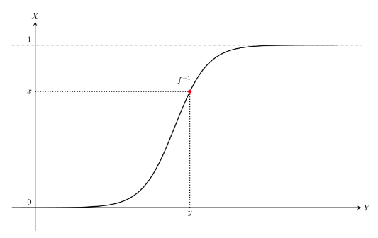
1. Create uniform distribution function by using Python algorithm
2. Create x numbers from uniform distribution function
3. Assign all x numbers into monotonous increasing function f(x)
4. Get y values
5. Suppose random variable Y which has set of y values
* $$$F_Y(y)=f^{-1}(x)$$$
 ================================================================================
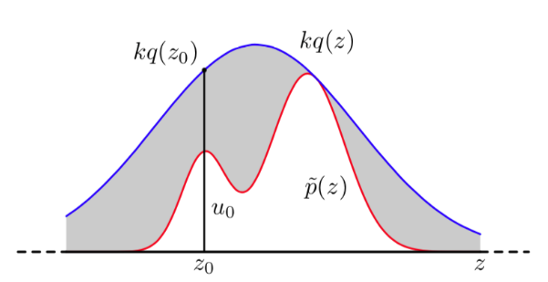
* Rejection sampling
- Suppose you have target probability distribution p(x) which you want to have
- Supposee there is probability distribution q(x) which is similar to p(x)
- But q(x) is easier to generate samples than q(x)
- Generate samples from q(x)
- You decide whether you throw extracted sample from q(x) away or not,
by using probability $$$\frac{p(z)}{kq(z)}$$$
- k is scaling constant to make $$$kq(x)\ge p(x)$$$
================================================================================
* Rejection sampling
- Suppose you have target probability distribution p(x) which you want to have
- Supposee there is probability distribution q(x) which is similar to p(x)
- But q(x) is easier to generate samples than q(x)
- Generate samples from q(x)
- You decide whether you throw extracted sample from q(x) away or not,
by using probability $$$\frac{p(z)}{kq(z)}$$$
- k is scaling constant to make $$$kq(x)\ge p(x)$$$
 ================================================================================
* Inference expectation value
* You can inference "expectation value" of probability distribution.
* It's the reason why you want to create samples from probability distribution
because you can inference expectation value of that probability distribution via sample
================================================================================
* Suppose you have probability distribution p(X) which you want to analyze
* Expectation value of p(X) is $$$\text{E}[f(X)] = \int f(x)p(x)dx$$$
* How to calculate (or inference) expectation value?
* Use monte carlo integration when you have N samples $$$\{ x_1, \ldots, x_N \}$$$
$$$\text{E}[f(X)] \approx \dfrac{1}{N} \sum_{i=1}^N f(x_i)$$$
* Error becomes smaller as you have larger N
================================================================================
* Importance sampling
- Suppose your goal is only to generate samples to calculate expectation value
- Then you can use importance sampling
- Importance sampling = generating samples + monte carlo integration for calculating expectation value
================================================================================
Step
- Create similar distribution q(x) which satisfies $$$kq(x)>p(x)$$$
- Calculate expectation value using following equation
$$$\text{E}[f(X)]
= \int f(x)p(x)dx \\
= \int f(x)\dfrac{p(x)}{q(x)} q(x) dx \\
\approx \dfrac{1}{N} \sum_{i=1}^N f(x_i)\dfrac{p(x_i)}{q(x_i)}$$$
================================================================================
* $$$\dfrac{p(x_i)}{q(x_i)}$$$ is called importance
because it is used as weight for samples
* There is less samples thrown away than rejection sampling
which threw away 80% of samples in above example.
================================================================================
* Markov chain
- Suppose time series probability procedure
- Suppose that time series probability procedure has K finite states
- If probability distribution $$$p(x_t) depends on p(x_{t-1}) and p(x_t|x_{t-1})$$$
this time series probability procedure is called "Markov chain"
- Note that "Markov chain" is different from "linear chain Markov network"
================================================================================
Let's apply "law of the total probability" on discrete state Markov chain
Then, following is true.
$$$p(x_{t}) = \sum_{x_{t-1}} p(x_t, x_{t-1}) = \sum_{x_{t-1}} p(x_t | x_{t-1}) p(x_{t-1})$$$
================================================================================
$$$p(x_t)$$$ is category distribution, you can express it as row vector $$$p_t$$$
then, you can convert $$$p(x_{t}) = \sum_{x_{t-1}} p(x_t, x_{t-1}) = \sum_{x_{t-1}} p(x_t | x_{t-1}) p(x_{t-1})$$$ to following matrix form
$$$p_t=p_{t-1}T$$$
$$$T$$$: transition matrix, $$$K\times K$$$ matrix, conditional probability
$$$T_{ij}=P(x_t=j|x_{t-1}=i)$$$
================================================================================
If transition matrix is symmetric matrix,
Markov chain is called "reversible Markov chain"
or you say Markov chain satisfies "detailed balance condition"
================================================================================
These Markov chain always converges into same distribution $$$p_{\infty}$$$
regardless of initial condition $$$p_0$$$ as time t goes by.
$$$p_{t'} = p_{t'+1} = p_{t'+2} = p_{t'+3} = \cdots = p_{\infty}$$$
$$$t'$$$: time after convergence
After reaching to convergence state,
samples $$$\{x_{t'}, x_{t'+1}, x_{t'+1}, \ldots, x_{t'+N} \}$$$ are independent values
which come from same probability distribution
================================================================================
MCMC
Markov Chain Monte Carlo generates samples using Markov chain.
You first create Markov chain for Markov chain's convergence distribution to have p(x)
Then, you run this Markov chain for $$$t^{'}$$$ hours,
after that, you can get samples in distribution you want.
================================================================================
Metropolis-Hastings Sampling
Metropolis-Hastings Sampling is used to generate sample as part method of MCMC.
Metropolis-Hastings Sampling is similar to rejection sampling
but MH uses conditional distribution $$$q(x^*|x_t)$$$ instead of unconditional distribution $$$q(x)$$$
for calculation distribution.
MH generally uses Gaussian distribution which has expectation value $$$x_t$$$
$$$q(x^*|x_t)=N(x^*|x_t,\sigma^2)$$$
================================================================================
How to generate samples using Metropolis-Hastings
- if $$$t=0$$$, randomly generate $$$x_t$$$
- generate sampe $$$x^*$$$ from distribution $$$q(x^*|x_t=x_t)$$$ where samples can be generated
- According to following probability p, select x_{t+1} for x^*
Following probability p is called Metropolis-Hastings criterion
$$$p = \min \left( 1, \dfrac{p(x^{\ast}) q(x_t \mid x^{\ast})}{p(x_t) q(x^{\ast} \mid x_t)} \right)$$$
If none is selected, newly selected value should be thrown away, you use previous value,
$$$x_{t+1}=x_t$$$
- You iterate above step until you have enough number of samples.
================================================================================
If calculation distribution $$$q(x^*|x_t)$$$ is Gaussian normal distribution,
if condition x_t and result $$$x^*$$$ are changed, probability is same.
$$$q(x^{\ast} \mid x_t) = q(x_t \mid x^{\ast})$$$
================================================================================
In this case, criterion becomes
$$$p = \min \left( 1, \dfrac{p(x^{\ast})}{p(x_t)} \right)$$$
which is called "Metropolis criterion"
================================================================================
According to Metropolis criterion,
it tries to make $$$p(x^*)$$$ bigger than $$$p(x_t)$$$
================================================================================
PyMC3 is used to generate MCMC samples and is used to perform Bayesian inference.
PyMC3 can use GPU
================================================================================
================================================================================
* Inference expectation value
* You can inference "expectation value" of probability distribution.
* It's the reason why you want to create samples from probability distribution
because you can inference expectation value of that probability distribution via sample
================================================================================
* Suppose you have probability distribution p(X) which you want to analyze
* Expectation value of p(X) is $$$\text{E}[f(X)] = \int f(x)p(x)dx$$$
* How to calculate (or inference) expectation value?
* Use monte carlo integration when you have N samples $$$\{ x_1, \ldots, x_N \}$$$
$$$\text{E}[f(X)] \approx \dfrac{1}{N} \sum_{i=1}^N f(x_i)$$$
* Error becomes smaller as you have larger N
================================================================================
* Importance sampling
- Suppose your goal is only to generate samples to calculate expectation value
- Then you can use importance sampling
- Importance sampling = generating samples + monte carlo integration for calculating expectation value
================================================================================
Step
- Create similar distribution q(x) which satisfies $$$kq(x)>p(x)$$$
- Calculate expectation value using following equation
$$$\text{E}[f(X)]
= \int f(x)p(x)dx \\
= \int f(x)\dfrac{p(x)}{q(x)} q(x) dx \\
\approx \dfrac{1}{N} \sum_{i=1}^N f(x_i)\dfrac{p(x_i)}{q(x_i)}$$$
================================================================================
* $$$\dfrac{p(x_i)}{q(x_i)}$$$ is called importance
because it is used as weight for samples
* There is less samples thrown away than rejection sampling
which threw away 80% of samples in above example.
================================================================================
* Markov chain
- Suppose time series probability procedure
- Suppose that time series probability procedure has K finite states
- If probability distribution $$$p(x_t) depends on p(x_{t-1}) and p(x_t|x_{t-1})$$$
this time series probability procedure is called "Markov chain"
- Note that "Markov chain" is different from "linear chain Markov network"
================================================================================
Let's apply "law of the total probability" on discrete state Markov chain
Then, following is true.
$$$p(x_{t}) = \sum_{x_{t-1}} p(x_t, x_{t-1}) = \sum_{x_{t-1}} p(x_t | x_{t-1}) p(x_{t-1})$$$
================================================================================
$$$p(x_t)$$$ is category distribution, you can express it as row vector $$$p_t$$$
then, you can convert $$$p(x_{t}) = \sum_{x_{t-1}} p(x_t, x_{t-1}) = \sum_{x_{t-1}} p(x_t | x_{t-1}) p(x_{t-1})$$$ to following matrix form
$$$p_t=p_{t-1}T$$$
$$$T$$$: transition matrix, $$$K\times K$$$ matrix, conditional probability
$$$T_{ij}=P(x_t=j|x_{t-1}=i)$$$
================================================================================
If transition matrix is symmetric matrix,
Markov chain is called "reversible Markov chain"
or you say Markov chain satisfies "detailed balance condition"
================================================================================
These Markov chain always converges into same distribution $$$p_{\infty}$$$
regardless of initial condition $$$p_0$$$ as time t goes by.
$$$p_{t'} = p_{t'+1} = p_{t'+2} = p_{t'+3} = \cdots = p_{\infty}$$$
$$$t'$$$: time after convergence
After reaching to convergence state,
samples $$$\{x_{t'}, x_{t'+1}, x_{t'+1}, \ldots, x_{t'+N} \}$$$ are independent values
which come from same probability distribution
================================================================================
MCMC
Markov Chain Monte Carlo generates samples using Markov chain.
You first create Markov chain for Markov chain's convergence distribution to have p(x)
Then, you run this Markov chain for $$$t^{'}$$$ hours,
after that, you can get samples in distribution you want.
================================================================================
Metropolis-Hastings Sampling
Metropolis-Hastings Sampling is used to generate sample as part method of MCMC.
Metropolis-Hastings Sampling is similar to rejection sampling
but MH uses conditional distribution $$$q(x^*|x_t)$$$ instead of unconditional distribution $$$q(x)$$$
for calculation distribution.
MH generally uses Gaussian distribution which has expectation value $$$x_t$$$
$$$q(x^*|x_t)=N(x^*|x_t,\sigma^2)$$$
================================================================================
How to generate samples using Metropolis-Hastings
- if $$$t=0$$$, randomly generate $$$x_t$$$
- generate sampe $$$x^*$$$ from distribution $$$q(x^*|x_t=x_t)$$$ where samples can be generated
- According to following probability p, select x_{t+1} for x^*
Following probability p is called Metropolis-Hastings criterion
$$$p = \min \left( 1, \dfrac{p(x^{\ast}) q(x_t \mid x^{\ast})}{p(x_t) q(x^{\ast} \mid x_t)} \right)$$$
If none is selected, newly selected value should be thrown away, you use previous value,
$$$x_{t+1}=x_t$$$
- You iterate above step until you have enough number of samples.
================================================================================
If calculation distribution $$$q(x^*|x_t)$$$ is Gaussian normal distribution,
if condition x_t and result $$$x^*$$$ are changed, probability is same.
$$$q(x^{\ast} \mid x_t) = q(x_t \mid x^{\ast})$$$
================================================================================
In this case, criterion becomes
$$$p = \min \left( 1, \dfrac{p(x^{\ast})}{p(x_t)} \right)$$$
which is called "Metropolis criterion"
================================================================================
According to Metropolis criterion,
it tries to make $$$p(x^*)$$$ bigger than $$$p(x_t)$$$
================================================================================
PyMC3 is used to generate MCMC samples and is used to perform Bayesian inference.
PyMC3 can use GPU
================================================================================
# @ Code
# If you already installed MKL library, you first need to execute this
import os
os.environ["MKL_THREADING_LAYER"]="GNU"

# ================================================================================
import pymc3 as pm
# @ Code
# c cov: covariance matrix
cov=np.array([[1.,1.5],[1.5,4]])
# c mu: mean value
mu=np.array([1,-1])

# ================================================================================
# Create Model scope
with pm.Model() as model:
  # c x: instance of multivariate Gaussian normal distribution
  x = pm.MvNormal('x',mu=mu,cov=cov,shape=(1,2))

  # c step: instance of Metropolis
  step = pm.Metropolis()

  # @ Execute generating 1000 sample
  trace = pm.sample(1000, step)

# ================================================================================
import warnings
warnings.simplefilter("ignore")

pm.traceplot(trace)
plt.show()

plt.scatter(trace['x'][:, 0, 0], trace['x'][:, 0, 1])
plt.show()
# @ Code
theta0=0.7

# @ Set seed number
np.random.seed(0)

# c x_data1: generated 10 data which follow bernoulli distribution
x_data1=sp.stats.bernoulli(theta0).rvs(10)
print(x_data1)
# array([1, 0, 1, 1, 1, 1, 1, 0, 0, 1])

# @ create model scope
with pm.Model() as model:
  theta=pm.Beta('theta',alpha=1,beta=1)

  x=pm.Bernoulli('x',p=theta,observed=x_data1)

  start=pm.find_MAP()

  step=pm.NUTS()

  trace1=pm.sample(2000,step=step,start=start)

pm.traceplot(trace1)
plt.show()

pm.plot_posterior(trace1)
plt.xlim(0, 1)
plt.show()
# @ Code
from sklearn.datasets import make_regression

# @ Create data for regression task
# 100 samples, 1 feature
x,y_data,coef=make_regression(n_samples=100,n_features=1,bias=0,noise=20,coef=True,random_state=1)
x = x.flatten()

# ================================================================================
print(coef)
# array(80.71051956)

# ================================================================================
plt.scatter(x, y_data)
plt.show()

# ================================================================================
# Create Model scope
with pm.Model() as m:

  w=pm.Normal('w',mu=0,sd=50)
  b=pm.Normal('b',mu=0,sd=50)
  esd=pm.HalfCauchy('esd',5)
  y=pm.Normal('y',mu=w*x+b,sd=esd,observed=y_data)

  start = pm.find_MAP()
  step = pm.NUTS()
  trace1 = pm.sample(10000, step=step, start=start)

# logp = -448.82, ||grad|| = 6.8486: 100%|██████████| 37/37 [00:00<00:00, 1599.20it/s]
# Multiprocess sampling (4 chains in 4 jobs)
# NUTS: [esd, b, w]
# Sampling 4 chains: 100%|██████████| 42000/42000 [00:16<00:00, 2477.73draws/s]

# ================================================================================
pm.traceplot(trace1)
plt.show()

# ================================================================================
pm.summary(trace1)