025-001. bernoulli distribution
@
In some trial, if result comes either success or fail, that trial is calls bernoulli trial
Example of bernoulli trial is coin toss
@
If you want to represent result of bernoulli trial in random variable X,
success is denoted by X=1,
fail is denoted by X=0
Sometimes, fail denoted by X=-1
@
Since bernoulli random variable has 0 or 1, bernoulli random variable is discrete random variable
Therefore, bernoulli distribution can be defined by probability mass function
@
probability mass function of bernoulli distribution is defined as follow
$Bern(x;\theta) = \theta$ if x = 1
$Bern(x;\theta) = 1 - \theta$ if x = 0
Bernoulli random variable has one parameter $\theta$ which means probability of occuring 1
Independent variable x and parameter $\theta$ are separated by ";"
Probability of occurring 0 is $1-\theta$
@
Above formular can be represented as one sentence
$Bern(x;\theta) = \theta^{x} (1 - \theta)^{(1-x)}$
@
Practice 1
1. In above one sentence formular, put x=1 and x=0, then check if you can get pmf of bernoulli distribution
@
If bernoulli random variable has 1 or -1,
you should denote bernoulli distribution as following
$Bern(x;\theta) = \theta^{\frac{(1+x)}{2}} (1-\theta)^{\frac{(1-x)}{2}}$
@
If some random variable X is occurred by bernoulli distribution,
we say random variable X follows bernoulli distribution
And we denote it in formular as follow
$X\sim Bern(x;\theta)$
@
SciPy를 사용한 베르누이 분포의 시뮬레이션
We can use bernoulli class in stats subpackage of scipy for bernoulli distribution
You can use argument p for parameter $\theta$
% I configure p = 0.6
theta = 0.6
rv = sp.stats.bernoulli(theta)
@
% You can calculate probability mass function by using pmf()
% This is values which X can have
xx = [0, 1]
% I get probability mass function of bernoulli distribution
plt.bar(xx, rv.pmf(xx))
plt.xlim(-1, 2)
plt.ylim(0, 1)
% Name of graph for 0 is x=0
plt.xticks([0, 1], ["x=0", "x=1"])
plt.xlabel("Sample values")
plt.ylabel("P(x)")
plt.title("pmf of bernoulli distribution")
plt.show()
#img 1195e5a1-8724-472e-990b-338c6a8daa6b
 @
% You can use rvs() to simulate trial
% 100 trials
x = rv.rvs(100, random_state=0)
x
% array([1, 0, 0, 1, 1, 0, 1, 0, 0, 1, 0, 1, 1, 0, 1, 1, 1, 0, 0, 0, 0, 0, 1,
% 0, 1, 0, 1, 0, 1, 1, 1, 0, 1, 1, 1, 0, 0, 0, 0, 0, 1, 1, 0, 1, 0, 0,
% 1, 1, 1, 1, 1, 1, 0, 1, 1, 1, 0, 1, 1, 1, 1, 1, 0, 1, 1, 1, 0, 1, 0,
% 1, 0, 1, 0, 0, 0, 1, 1, 1, 1, 1, 1, 1, 1, 0, 1, 1, 1, 1, 1, 0, 1, 0,
% 1, 0, 1, 1, 1, 1, 0, 1])
@
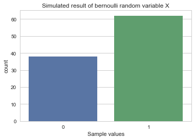
% I can visualize simulated result by using countplot() of seaborn package
% I pass simulated data x
sns.countplot(x)
plt.title("Simulated result of bernoulli random variable X")
plt.xlabel("Sample values")
plt.show()
#img d5ea3c80-4331-4fae-b846-6dcc569b84e5
@
% You can use rvs() to simulate trial
% 100 trials
x = rv.rvs(100, random_state=0)
x
% array([1, 0, 0, 1, 1, 0, 1, 0, 0, 1, 0, 1, 1, 0, 1, 1, 1, 0, 0, 0, 0, 0, 1,
% 0, 1, 0, 1, 0, 1, 1, 1, 0, 1, 1, 1, 0, 0, 0, 0, 0, 1, 1, 0, 1, 0, 0,
% 1, 1, 1, 1, 1, 1, 0, 1, 1, 1, 0, 1, 1, 1, 1, 1, 0, 1, 1, 1, 0, 1, 0,
% 1, 0, 1, 0, 0, 0, 1, 1, 1, 1, 1, 1, 1, 1, 0, 1, 1, 1, 1, 1, 0, 1, 0,
% 1, 0, 1, 1, 1, 1, 0, 1])
@
% I can visualize simulated result by using countplot() of seaborn package
% I pass simulated data x
sns.countplot(x)
plt.title("Simulated result of bernoulli random variable X")
plt.xlabel("Sample values")
plt.show()
#img d5ea3c80-4331-4fae-b846-6dcc569b84e5
 @
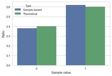
% You can use following code to show both theoretical probability distribtion and sample based probability distribtion
% x = rv.rvs(100, random_state=0)
y = np.bincount(x, minlength=2) / float(len(x))
% count of 1 and 0 / 100.0
% array([38, 62], dtype=int64) / 100.0
% array([0.38, 0.62])
% I make dataframe
df = pd.DataFrame({"Theoretical":rv.pmf(xx), "Sample based":y})
df
% Sample based Theoretical
% 0 0.38 0.4
% 1 0.62 0.6
% You can visualize above result by using barplot() of seaborn
% First, I reset index for df
df2 = df.stack().reset_index()
% I set columns by list of data
df2.columns = ["Sample value", "Type", "Ratio"]
df2
% Sample value Type Ratio
% 0 0 Sample based 0.38
% 1 0 Theoretical 0.40
% 2 1 Sample based 0.62
% 3 1 Theoretical 0.60
% I use barplot()
% I configure barplot
sns.barplot(x="Sample value", y="Ratio", hue="Type", data=df2)
plt.show()
#img 908c0b45-5892-4504-8c88-ce5c940d3a1e
@
% You can use following code to show both theoretical probability distribtion and sample based probability distribtion
% x = rv.rvs(100, random_state=0)
y = np.bincount(x, minlength=2) / float(len(x))
% count of 1 and 0 / 100.0
% array([38, 62], dtype=int64) / 100.0
% array([0.38, 0.62])
% I make dataframe
df = pd.DataFrame({"Theoretical":rv.pmf(xx), "Sample based":y})
df
% Sample based Theoretical
% 0 0.38 0.4
% 1 0.62 0.6
% You can visualize above result by using barplot() of seaborn
% First, I reset index for df
df2 = df.stack().reset_index()
% I set columns by list of data
df2.columns = ["Sample value", "Type", "Ratio"]
df2
% Sample value Type Ratio
% 0 0 Sample based 0.38
% 1 0 Theoretical 0.40
% 2 1 Sample based 0.62
% 3 1 Theoretical 0.60
% I use barplot()
% I configure barplot
sns.barplot(x="Sample value", y="Ratio", hue="Type", data=df2)
plt.show()
#img 908c0b45-5892-4504-8c88-ce5c940d3a1e
 @
Moments of bernoulli distribtion are as following
1. Expectation of X
$E[X]=\theta$
(proof)
$E[X] = \sum x_{i}P(x_{i})$
$E[X] = 1\cdot\theta + 0\cdot(1-\theta)$
$E[X] = \theta$
2. Variance of X
$Var[X] = \theta(1-\theta)$
(proof)
$Var[X] = \sum(x_{i}-\mu)^{2} P(x_{i})$
$Var[X] = (1-\theta)^{2}\cdot\theta+(0-\theta)^{2}\cdot(1-\theta)$
$Var[X] = \theta(1-\theta)$
In above example, $\theta = 0.6$
So, theoretical expection of X and variance of X are following ones
E[X]=0.6
$Var[X]=0.6\cdot(1-0.6)=0.24$
@
% You can calculate sample mean and sample variance as following
np.mean(x)
% 0.62
np.var(x, ddof=1)
% 0.23797979797979804
@
% You can use describe() of scipy
s = sp.stats.describe(x)
s[0], s[1]
% (100, (0, 1))
% mean of x, variance of x
s[2], s[3]
% (0.62, 0.23797979797979804)
@
Practice 2
1. Find expection of X and variance of X with parameter $\theta = 0.5$
Draw countplot compared with pmf
Calculate above calculation with 10 sample and 1000 samples
2. Find expection of X and variance of X with parameter $\theta = 0.9$
Draw countplot compared with pmf
Calculate above calculation with 10 sample and 1000 samples
@
We can find parameter from sample data
Above step is called parameter estimation
In case of bernoulli distribtion, we can estimate its parameter as following
$\hat{\theta} = \frac{\sum\limits_{i=1}^{N}x_{i}}{N}$
$\hat{\theta} = \frac{N_{1}}{N}$
$\hat{\theta}$ : estimated parameter
N : the number of sample data
$N_{1}$ : the number of occurring 1
@
% You can apply bernoulli distribtion in following cases
% 1. When output data of classification prediction question is categorical value having 2 values
% You can use bernoulli distribtion to represent which category value has high likelihood
% 1. 1. When input data is categorical value having 2 values, you can use bernoulli distribtion to represent ratio of showing each value
@
% Suppose you made spam filter which distinguishes ham and spam
% Suppose you get 10 emails
% Suppose 6 are spam and 4 are ham
% We can judge one email coming can be spam with 60%
% This case can be represented by bernoulli distribtion with $\theta=0.6$
$P(Y)=Bern(y;\theta=0.6)$
% Random variable Y represents if arrived email is spam or no
% If Y=1 occurs, it means spam
% Spam email has high likelihood of having specific kind of word and keyword
% If you have various keyword to distinguish spam and ham, you can represent those keywords in form of BOW which is encoded vector
% In this case, we suppose spam keywords are composed of 4 words
$\begin{bmatrix} 1\\0\\1\\0 \end{bmatrix}$
% Above vector means this email has 1st keyword and 3rd keyword of spam keywords
% If you have 6 emails, you can represent like this
$\begin{bmatrix} 1&0&1&0 \\ 1&1&1&0 \\ 1&1&0&1 \\ 0&0&1&1 \\ 1&1&0&0 \\ 1&1&0&1 \end{bmatrix}$
In this case, we can represent characteristic of spam email in 4 bernoulli distribtions($X_{1}, X_{2}, X_{3}, X_{4}$)
$X_{1} \sim Bern(x_{1} ; \theta_{1})$ : probability that spam email has 1st keyword
$X_{2} \sim Bern(x_{2} ; \theta_{2})$ : probability that spam email has 2nd keyword
$X_{3} \sim Bern(x_{3} ; \theta_{3})$ : probability that spam email has 3rd keyword
$X_{4} \sim Bern(x_{4} ; \theta_{4})$ : probability that spam email has 4th keyword
We suppose each parameter for each bernoulli distribtion
$\theta_{1} = \frac{5}{6}$
$\theta_{2} = \frac{4}{6}$
$\theta_{3} = \frac{3}{6}$
$\theta_{4} = \frac{3}{6}$
@
% Practice 3
% If ham email represents as following, how can you represent characteristic of ham email?
$\begin{bmatrix} 0&0&1&1 \\ 0&1&1&1 \\ 0&0&1&1 \\ 1&0&0&1 \end{bmatrix}$
@
Moments of bernoulli distribtion are as following
1. Expectation of X
$E[X]=\theta$
(proof)
$E[X] = \sum x_{i}P(x_{i})$
$E[X] = 1\cdot\theta + 0\cdot(1-\theta)$
$E[X] = \theta$
2. Variance of X
$Var[X] = \theta(1-\theta)$
(proof)
$Var[X] = \sum(x_{i}-\mu)^{2} P(x_{i})$
$Var[X] = (1-\theta)^{2}\cdot\theta+(0-\theta)^{2}\cdot(1-\theta)$
$Var[X] = \theta(1-\theta)$
In above example, $\theta = 0.6$
So, theoretical expection of X and variance of X are following ones
E[X]=0.6
$Var[X]=0.6\cdot(1-0.6)=0.24$
@
% You can calculate sample mean and sample variance as following
np.mean(x)
% 0.62
np.var(x, ddof=1)
% 0.23797979797979804
@
% You can use describe() of scipy
s = sp.stats.describe(x)
s[0], s[1]
% (100, (0, 1))
% mean of x, variance of x
s[2], s[3]
% (0.62, 0.23797979797979804)
@
Practice 2
1. Find expection of X and variance of X with parameter $\theta = 0.5$
Draw countplot compared with pmf
Calculate above calculation with 10 sample and 1000 samples
2. Find expection of X and variance of X with parameter $\theta = 0.9$
Draw countplot compared with pmf
Calculate above calculation with 10 sample and 1000 samples
@
We can find parameter from sample data
Above step is called parameter estimation
In case of bernoulli distribtion, we can estimate its parameter as following
$\hat{\theta} = \frac{\sum\limits_{i=1}^{N}x_{i}}{N}$
$\hat{\theta} = \frac{N_{1}}{N}$
$\hat{\theta}$ : estimated parameter
N : the number of sample data
$N_{1}$ : the number of occurring 1
@
% You can apply bernoulli distribtion in following cases
% 1. When output data of classification prediction question is categorical value having 2 values
% You can use bernoulli distribtion to represent which category value has high likelihood
% 1. 1. When input data is categorical value having 2 values, you can use bernoulli distribtion to represent ratio of showing each value
@
% Suppose you made spam filter which distinguishes ham and spam
% Suppose you get 10 emails
% Suppose 6 are spam and 4 are ham
% We can judge one email coming can be spam with 60%
% This case can be represented by bernoulli distribtion with $\theta=0.6$
$P(Y)=Bern(y;\theta=0.6)$
% Random variable Y represents if arrived email is spam or no
% If Y=1 occurs, it means spam
% Spam email has high likelihood of having specific kind of word and keyword
% If you have various keyword to distinguish spam and ham, you can represent those keywords in form of BOW which is encoded vector
% In this case, we suppose spam keywords are composed of 4 words
$\begin{bmatrix} 1\\0\\1\\0 \end{bmatrix}$
% Above vector means this email has 1st keyword and 3rd keyword of spam keywords
% If you have 6 emails, you can represent like this
$\begin{bmatrix} 1&0&1&0 \\ 1&1&1&0 \\ 1&1&0&1 \\ 0&0&1&1 \\ 1&1&0&0 \\ 1&1&0&1 \end{bmatrix}$
In this case, we can represent characteristic of spam email in 4 bernoulli distribtions($X_{1}, X_{2}, X_{3}, X_{4}$)
$X_{1} \sim Bern(x_{1} ; \theta_{1})$ : probability that spam email has 1st keyword
$X_{2} \sim Bern(x_{2} ; \theta_{2})$ : probability that spam email has 2nd keyword
$X_{3} \sim Bern(x_{3} ; \theta_{3})$ : probability that spam email has 3rd keyword
$X_{4} \sim Bern(x_{4} ; \theta_{4})$ : probability that spam email has 4th keyword
We suppose each parameter for each bernoulli distribtion
$\theta_{1} = \frac{5}{6}$
$\theta_{2} = \frac{4}{6}$
$\theta_{3} = \frac{3}{6}$
$\theta_{4} = \frac{3}{6}$
@
% Practice 3
% If ham email represents as following, how can you represent characteristic of ham email?
$\begin{bmatrix} 0&0&1&1 \\ 0&1&1&1 \\ 0&0&1&1 \\ 1&0&0&1 \end{bmatrix}$