045-001. K-Means clustring
@
You don't predict y value from data
You make each cluster by using features of independent variable x
This is called clustring
@
K-Means clustring algorithm is one of simplest and fastest clustering algorithms
First, you find target function
You couninuously find the number of clusters K and centroid of each cluster $\mu_{K}$ until target function goes lowest
Target function $J = \sum\limits_{K=1}^{K} \sum\limits_{i\in C_{K}} d(x_{i}, \mu_{k})$
$d(x_{i}, \mu_{k})$ is similarity function or distance between two data
$d(x_{i}, \mu_{k}) = ||x_{i}−\mu_K||^{2}$
@
Following is detailed steps for k-means clustering algorithm
1. You choose random centroid $\mu_{k}$ (generally, you randomly choose one from data sample)
2. You calculate distance between centroid and each indivitual data of sample
3. You choose nearest centroid from each data, and based on this, you update boundary group of cluster
4. You calculate centroid from newly updated cluster, and iterate step 1 to step 4
@
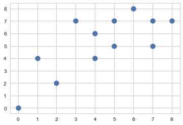
X = np.array([[7, 5],[5, 7],[7, 7],[4, 4],[4, 6],[1, 4],[0, 0],[2, 2],[8, 7],[6, 8],[5, 5],[3, 7]])
plt.scatter(X[:,0], X[:,1], s=100)
plt.show()
#img 045-001-001
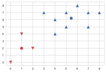
 from sklearn.cluster import KMeans
model = KMeans(n_clusters=2, init="random", n_init=1, max_iter=1, random_state=1).fit(X)
c0, c1 = model.cluster_centers_
print(c0, c1)
plt.scatter(X[model.labels_==0,0], X[model.labels_==0,1], s=100, marker='v', c='r')
plt.scatter(X[model.labels_==1,0], X[model.labels_==1,1], s=100, marker='^', c='b')
plt.scatter(c0[0], c0[1], s=100, c="r")
plt.scatter(c1[0], c1[1], s=100, c="b")
plt.show()
#img 045-001-002
% [6.6 6.8] [2.71428571 4. ]
from sklearn.cluster import KMeans
model = KMeans(n_clusters=2, init="random", n_init=1, max_iter=1, random_state=1).fit(X)
c0, c1 = model.cluster_centers_
print(c0, c1)
plt.scatter(X[model.labels_==0,0], X[model.labels_==0,1], s=100, marker='v', c='r')
plt.scatter(X[model.labels_==1,0], X[model.labels_==1,1], s=100, marker='^', c='b')
plt.scatter(c0[0], c0[1], s=100, c="r")
plt.scatter(c1[0], c1[1], s=100, c="b")
plt.show()
#img 045-001-002
% [6.6 6.8] [2.71428571 4. ]
 def kmeans_df(c0, c1):
df = pd.DataFrame(np.hstack([X,
np.linalg.norm(X - c0, axis=1)[:, np.newaxis],
np.linalg.norm(X - c1, axis=1)[:, np.newaxis],
model.labels_[:, np.newaxis]]),
columns=["x0", "x1", "d0", "d1", "c"])
return df
kmeans_df(c0, c1)
% x0 x1 d0 d1 c
% 0 7.0 5.0 6.708204 1.978277 0.0
% 1 5.0 7.0 6.403124 0.895806 0.0
% 2 7.0 7.0 7.810250 1.739164 0.0
% 3 4.0 4.0 3.605551 2.650413 1.0
% 4 4.0 6.0 5.000000 1.461438 1.0
% 5 1.0 4.0 2.000000 4.969040 1.0
% 6 0.0 0.0 2.236068 8.267891 1.0
% 7 2.0 2.0 1.000000 5.448978 1.0
% 8 8.0 7.0 8.602325 2.671292 0.0
% 9 6.0 8.0 7.810250 1.862562 0.0
% 10 5.0 5.0 5.000000 1.300522 0.0
% 11 3.0 7.0 5.385165 2.565199 1.0
print(X[model.labels_==0,0].mean(), X[model.labels_==0,1].mean())
print(X[model.labels_==1,0].mean(), X[model.labels_==1,1].mean())
% 6.333333333333333 6.5
% 2.3333333333333335 3.8333333333333335
model.score(X)
% -63.00408163265304
model = KMeans(n_clusters=2, init="random", n_init=1, max_iter=2, random_state=0).fit(X)
c0, c1 = model.cluster_centers_
print(c0, c1)
plt.scatter(X[model.labels_==0,0], X[model.labels_==0,1], s=100, marker='v', c='r')
plt.scatter(X[model.labels_==1,0], X[model.labels_==1,1], s=100, marker='^', c='b')
plt.scatter(c0[0], c0[1], s=100, c="r")
plt.scatter(c1[0], c1[1], s=100, c="b")
kmeans_df(c0, c1)
#img 045-001-003
% [1. 2.] [5.44444444 6.22222222]
% x0 x1 d0 d1 c
% 0 7.0 5.0 6.708204 1.978277 1.0
% 1 5.0 7.0 6.403124 0.895806 1.0
% 2 7.0 7.0 7.810250 1.739164 1.0
% 3 4.0 4.0 3.605551 2.650413 1.0
% 4 4.0 6.0 5.000000 1.461438 1.0
% 5 1.0 4.0 2.000000 4.969040 0.0
% 6 0.0 0.0 2.236068 8.267891 0.0
% 7 2.0 2.0 1.000000 5.448978 0.0
% 8 8.0 7.0 8.602325 2.671292 1.0
% 9 6.0 8.0 7.810250 1.862562 1.0
% 10 5.0 5.0 5.000000 1.300522 1.0
% 11 3.0 7.0 5.385165 2.565199 1.0
def kmeans_df(c0, c1):
df = pd.DataFrame(np.hstack([X,
np.linalg.norm(X - c0, axis=1)[:, np.newaxis],
np.linalg.norm(X - c1, axis=1)[:, np.newaxis],
model.labels_[:, np.newaxis]]),
columns=["x0", "x1", "d0", "d1", "c"])
return df
kmeans_df(c0, c1)
% x0 x1 d0 d1 c
% 0 7.0 5.0 6.708204 1.978277 0.0
% 1 5.0 7.0 6.403124 0.895806 0.0
% 2 7.0 7.0 7.810250 1.739164 0.0
% 3 4.0 4.0 3.605551 2.650413 1.0
% 4 4.0 6.0 5.000000 1.461438 1.0
% 5 1.0 4.0 2.000000 4.969040 1.0
% 6 0.0 0.0 2.236068 8.267891 1.0
% 7 2.0 2.0 1.000000 5.448978 1.0
% 8 8.0 7.0 8.602325 2.671292 0.0
% 9 6.0 8.0 7.810250 1.862562 0.0
% 10 5.0 5.0 5.000000 1.300522 0.0
% 11 3.0 7.0 5.385165 2.565199 1.0
print(X[model.labels_==0,0].mean(), X[model.labels_==0,1].mean())
print(X[model.labels_==1,0].mean(), X[model.labels_==1,1].mean())
% 6.333333333333333 6.5
% 2.3333333333333335 3.8333333333333335
model.score(X)
% -63.00408163265304
model = KMeans(n_clusters=2, init="random", n_init=1, max_iter=2, random_state=0).fit(X)
c0, c1 = model.cluster_centers_
print(c0, c1)
plt.scatter(X[model.labels_==0,0], X[model.labels_==0,1], s=100, marker='v', c='r')
plt.scatter(X[model.labels_==1,0], X[model.labels_==1,1], s=100, marker='^', c='b')
plt.scatter(c0[0], c0[1], s=100, c="r")
plt.scatter(c1[0], c1[1], s=100, c="b")
kmeans_df(c0, c1)
#img 045-001-003
% [1. 2.] [5.44444444 6.22222222]
% x0 x1 d0 d1 c
% 0 7.0 5.0 6.708204 1.978277 1.0
% 1 5.0 7.0 6.403124 0.895806 1.0
% 2 7.0 7.0 7.810250 1.739164 1.0
% 3 4.0 4.0 3.605551 2.650413 1.0
% 4 4.0 6.0 5.000000 1.461438 1.0
% 5 1.0 4.0 2.000000 4.969040 0.0
% 6 0.0 0.0 2.236068 8.267891 0.0
% 7 2.0 2.0 1.000000 5.448978 0.0
% 8 8.0 7.0 8.602325 2.671292 1.0
% 9 6.0 8.0 7.810250 1.862562 1.0
% 10 5.0 5.0 5.000000 1.300522 1.0
% 11 3.0 7.0 5.385165 2.565199 1.0
 model.score(X)
% -45.777777777777715
(np.linalg.norm(X[model.labels_==0] - c0, axis=1)**2).sum() + \
(np.linalg.norm(X[model.labels_==1] - c1, axis=1)**2).sum()
% 45.77777777777778
model = KMeans(n_clusters=2, init="random", n_init=1, max_iter=100, random_state=0).fit(X)
c0, c1 = model.cluster_centers_
print(c0, c1)
plt.scatter(X[model.labels_==0,0], X[model.labels_==0,1], s=100, marker='v', c='r')
plt.scatter(X[model.labels_==1,0], X[model.labels_==1,1], s=100, marker='^', c='b')
plt.scatter(c0[0], c0[1], s=100, c="r")
plt.scatter(c1[0], c1[1], s=100, c="b")
kmeans_df(c0, c1)
#img 045-001-004
% [1. 2.] [5.44444444 6.22222222]
% x0 x1 d0 d1 c
% 0 7.0 5.0 6.708204 1.978277 1.0
% 1 5.0 7.0 6.403124 0.895806 1.0
% 2 7.0 7.0 7.810250 1.739164 1.0
% 3 4.0 4.0 3.605551 2.650413 1.0
% 4 4.0 6.0 5.000000 1.461438 1.0
% 5 1.0 4.0 2.000000 4.969040 0.0
% 6 0.0 0.0 2.236068 8.267891 0.0
% 7 2.0 2.0 1.000000 5.448978 0.0
% 8 8.0 7.0 8.602325 2.671292 1.0
% 9 6.0 8.0 7.810250 1.862562 1.0
% 10 5.0 5.0 5.000000 1.300522 1.0
% 11 3.0 7.0 5.385165 2.565199 1.0
model.score(X)
% -45.777777777777715
(np.linalg.norm(X[model.labels_==0] - c0, axis=1)**2).sum() + \
(np.linalg.norm(X[model.labels_==1] - c1, axis=1)**2).sum()
% 45.77777777777778
model = KMeans(n_clusters=2, init="random", n_init=1, max_iter=100, random_state=0).fit(X)
c0, c1 = model.cluster_centers_
print(c0, c1)
plt.scatter(X[model.labels_==0,0], X[model.labels_==0,1], s=100, marker='v', c='r')
plt.scatter(X[model.labels_==1,0], X[model.labels_==1,1], s=100, marker='^', c='b')
plt.scatter(c0[0], c0[1], s=100, c="r")
plt.scatter(c1[0], c1[1], s=100, c="b")
kmeans_df(c0, c1)
#img 045-001-004
% [1. 2.] [5.44444444 6.22222222]
% x0 x1 d0 d1 c
% 0 7.0 5.0 6.708204 1.978277 1.0
% 1 5.0 7.0 6.403124 0.895806 1.0
% 2 7.0 7.0 7.810250 1.739164 1.0
% 3 4.0 4.0 3.605551 2.650413 1.0
% 4 4.0 6.0 5.000000 1.461438 1.0
% 5 1.0 4.0 2.000000 4.969040 0.0
% 6 0.0 0.0 2.236068 8.267891 0.0
% 7 2.0 2.0 1.000000 5.448978 0.0
% 8 8.0 7.0 8.602325 2.671292 1.0
% 9 6.0 8.0 7.810250 1.862562 1.0
% 10 5.0 5.0 5.000000 1.300522 1.0
% 11 3.0 7.0 5.385165 2.565199 1.0
 @
K-Means++ is algorithm to configure initial centroid
1. You prepare set M to store centroid in it
2. First of all, you choose one random centroid $\mu_{0}$ and store it into M
3. You calculate distance $d(M, x_{i})$ between M and $x_{i}$ which is all sample not involved in M
You can calculate $d(M, x_{i})$ by choosing minimal value from $d(\mu_{k}, x_{i})$ which is distance between $\mu_{k}$ which is all sample involved in M and $x_{i}$ which is all sample not involved in M
4. You choose next centroid $\mu$ based on probability which is proportional to $d(M, x_{i})$
5. You iterate above steps until you choose k number of centorid
6. With initialized centroid, you use k-means algorithm
@
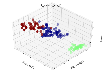
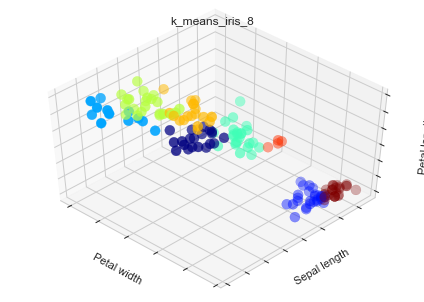
Let's deal with Iris data with k-means and k-means++
from mpl_toolkits.mplot3d import Axes3D
from sklearn.cluster import KMeans
from sklearn import datasets
np.random.seed(5)
centers = [[1, 1], [-1, -1], [1, -1]]
iris = datasets.load_iris()
X = iris.data
y = iris.target
estimators = {'k_means_iris_3': KMeans(n_clusters=3),
'k_means_iris_8': KMeans(n_clusters=8)}
fignum = 1
for name, est in estimators.items():
fig = plt.figure(fignum)
plt.clf()
ax = Axes3D(fig, rect=[0, 0, .95, 1], elev=48, azim=134)
plt.cla()
est.fit(X)
labels = est.labels_
ax.scatter(X[:, 3], X[:, 0], X[:, 2], c=labels.astype(np.float), s=100, cmap=mpl.cm.jet)
ax.w_xaxis.set_ticklabels([])
ax.w_yaxis.set_ticklabels([])
ax.w_zaxis.set_ticklabels([])
ax.set_xlabel('Petal width')
ax.set_ylabel('Sepal length')
ax.set_zlabel('Petal length')
plt.title(name)
fignum = fignum + 1
plt.show()
#img 045-001-005
#img 045-001-006
@
K-Means++ is algorithm to configure initial centroid
1. You prepare set M to store centroid in it
2. First of all, you choose one random centroid $\mu_{0}$ and store it into M
3. You calculate distance $d(M, x_{i})$ between M and $x_{i}$ which is all sample not involved in M
You can calculate $d(M, x_{i})$ by choosing minimal value from $d(\mu_{k}, x_{i})$ which is distance between $\mu_{k}$ which is all sample involved in M and $x_{i}$ which is all sample not involved in M
4. You choose next centroid $\mu$ based on probability which is proportional to $d(M, x_{i})$
5. You iterate above steps until you choose k number of centorid
6. With initialized centroid, you use k-means algorithm
@
Let's deal with Iris data with k-means and k-means++
from mpl_toolkits.mplot3d import Axes3D
from sklearn.cluster import KMeans
from sklearn import datasets
np.random.seed(5)
centers = [[1, 1], [-1, -1], [1, -1]]
iris = datasets.load_iris()
X = iris.data
y = iris.target
estimators = {'k_means_iris_3': KMeans(n_clusters=3),
'k_means_iris_8': KMeans(n_clusters=8)}
fignum = 1
for name, est in estimators.items():
fig = plt.figure(fignum)
plt.clf()
ax = Axes3D(fig, rect=[0, 0, .95, 1], elev=48, azim=134)
plt.cla()
est.fit(X)
labels = est.labels_
ax.scatter(X[:, 3], X[:, 0], X[:, 2], c=labels.astype(np.float), s=100, cmap=mpl.cm.jet)
ax.w_xaxis.set_ticklabels([])
ax.w_yaxis.set_ticklabels([])
ax.w_zaxis.set_ticklabels([])
ax.set_xlabel('Petal width')
ax.set_ylabel('Sepal length')
ax.set_zlabel('Petal length')
plt.title(name)
fignum = fignum + 1
plt.show()
#img 045-001-005
#img 045-001-006
 @
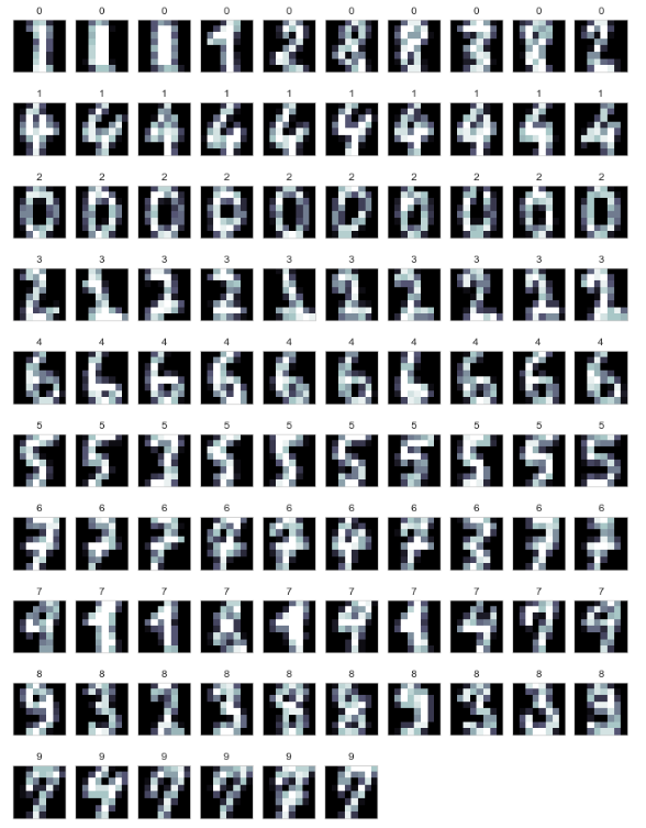
Let's deal with Digit Image with k-means and k-means++
from sklearn.datasets import load_digits
from sklearn.preprocessing import scale
digits = load_digits()
data = scale(digits.data)
def print_digits(images, labels):
f = plt.figure(figsize=(10,2))
plt.subplots_adjust(top=1, bottom=0, hspace=0, wspace=0.05)
i = 0
while (i < 10 and i < images.shape[0]):
ax = f.add_subplot(1, 10, i + 1)
ax.imshow(images[i], cmap=plt.cm.bone)
ax.grid(False)
ax.table
ax.set_title(labels[i])
ax.xaxis.set_ticks([])
ax.yaxis.set_ticks([])
plt.tight_layout()
i += 1
print_digits(digits.images, range(10))
#img 1195e5a1-8724-472e-990b-338c6a8daa6b
@
Let's deal with Digit Image with k-means and k-means++
from sklearn.datasets import load_digits
from sklearn.preprocessing import scale
digits = load_digits()
data = scale(digits.data)
def print_digits(images, labels):
f = plt.figure(figsize=(10,2))
plt.subplots_adjust(top=1, bottom=0, hspace=0, wspace=0.05)
i = 0
while (i < 10 and i < images.shape[0]):
ax = f.add_subplot(1, 10, i + 1)
ax.imshow(images[i], cmap=plt.cm.bone)
ax.grid(False)
ax.table
ax.set_title(labels[i])
ax.xaxis.set_ticks([])
ax.yaxis.set_ticks([])
plt.tight_layout()
i += 1
print_digits(digits.images, range(10))
#img 1195e5a1-8724-472e-990b-338c6a8daa6b
 from sklearn.model_selection import train_test_split
X_train, X_test, y_train, y_test, images_train, images_test = \
train_test_split(data, digits.target, digits.images, test_size=0.25, random_state=42)
from sklearn.cluster import KMeans
clf = KMeans(init="k-means++", n_clusters=10, random_state=42)
clf.fit(X_train)
print_digits(images_train, clf.labels_)
#img 2eeb3735-ee7b-4c9e-912d-87a4b611f4ed
from sklearn.model_selection import train_test_split
X_train, X_test, y_train, y_test, images_train, images_test = \
train_test_split(data, digits.target, digits.images, test_size=0.25, random_state=42)
from sklearn.cluster import KMeans
clf = KMeans(init="k-means++", n_clusters=10, random_state=42)
clf.fit(X_train)
print_digits(images_train, clf.labels_)
#img 2eeb3735-ee7b-4c9e-912d-87a4b611f4ed
 y_pred = clf.predict(X_test)
def print_cluster(images, y_pred, cluster_number):
images = images[y_pred == cluster_number]
y_pred = y_pred[y_pred == cluster_number]
print_digits(images, y_pred)
for i in range(10):
print_cluster(images_test, y_pred, i)
#img 7fe8cafd-06bd-44e9-9ebc-9f24846465d7
from sklearn.metrics import confusion_matrix
confusion_matrix(y_test, y_pred)
array([[ 0, 0, 43, 0, 0, 0, 0, 0, 0, 0],
[20, 0, 0, 7, 0, 0, 0, 10, 0, 0],
[ 5, 0, 0, 31, 0, 0, 0, 1, 1, 0],
[ 1, 0, 0, 1, 0, 1, 4, 0, 39, 0],
[ 1, 50, 0, 0, 0, 0, 1, 2, 0, 1],
[ 1, 0, 0, 0, 1, 41, 0, 0, 16, 0],
[ 0, 0, 1, 0, 44, 0, 0, 0, 0, 0],
[ 0, 0, 0, 0, 0, 1, 34, 1, 0, 5],
[21, 0, 0, 0, 0, 3, 1, 2, 11, 0],
[ 0, 0, 0, 0, 0, 2, 3, 3, 40, 0]], dtype=int64)
y_pred = clf.predict(X_test)
def print_cluster(images, y_pred, cluster_number):
images = images[y_pred == cluster_number]
y_pred = y_pred[y_pred == cluster_number]
print_digits(images, y_pred)
for i in range(10):
print_cluster(images_test, y_pred, i)
#img 7fe8cafd-06bd-44e9-9ebc-9f24846465d7
from sklearn.metrics import confusion_matrix
confusion_matrix(y_test, y_pred)
array([[ 0, 0, 43, 0, 0, 0, 0, 0, 0, 0],
[20, 0, 0, 7, 0, 0, 0, 10, 0, 0],
[ 5, 0, 0, 31, 0, 0, 0, 1, 1, 0],
[ 1, 0, 0, 1, 0, 1, 4, 0, 39, 0],
[ 1, 50, 0, 0, 0, 0, 1, 2, 0, 1],
[ 1, 0, 0, 0, 1, 41, 0, 0, 16, 0],
[ 0, 0, 1, 0, 44, 0, 0, 0, 0, 0],
[ 0, 0, 0, 0, 0, 1, 34, 1, 0, 5],
[21, 0, 0, 0, 0, 3, 1, 2, 11, 0],
[ 0, 0, 0, 0, 0, 2, 3, 3, 40, 0]], dtype=int64)
 @
You can evaluate performance of clustring by following criterions
1. When you know exact answer(the number of clusters and belong), you can use
Adjusted Rand index
Adjusted Mutual Information
Homogeneity, completeness and V-measure
Fowlkes-Mallows scores
1. When you don't know exact answer(the number of clusters and belong), you can use
Silhouette Coefficient
Calinski-Harabaz Index
@
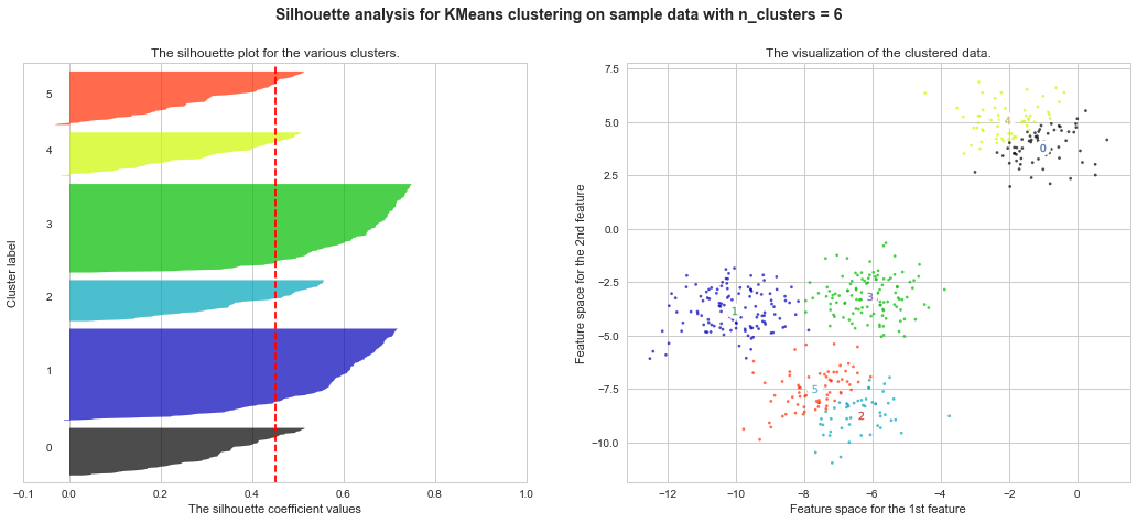
Example of silhouette coefficient
$s = \frac{b−a}{max(a,b)}$
a : average distance between each element inside of cluster
b : average distance of nearest distance between one element and other cluster's centroid
http://scikit-learn.org/stable/auto_examples/cluster/plot_kmeans_silhouette_analysis.html
from sklearn.datasets import make_blobs
from sklearn.cluster import KMeans
from sklearn.metrics import silhouette_samples, silhouette_score
import matplotlib.cm as cm
# Generating the sample data from make_blobs
# This particular setting has one distinct cluster and 3 clusters placed close
# together.
X, y = make_blobs(n_samples=500,
n_features=2,
centers=4,
cluster_std=1,
center_box=(-10.0, 10.0),
shuffle=True,
random_state=1) # For reproducibility
range_n_clusters = [2, 3, 4, 5, 6]
for n_clusters in range_n_clusters:
# Create a subplot with 1 row and 2 columns
fig, (ax1, ax2) = plt.subplots(1, 2)
fig.set_size_inches(18, 7)
# The 1st subplot is the silhouette plot
# The silhouette coefficient can range from -1, 1 but in this example all
# lie within [-0.1, 1]
ax1.set_xlim([-0.1, 1])
# The (n_clusters+1)*10 is for inserting blank space between silhouette
# plots of individual clusters, to demarcate them clearly.
ax1.set_ylim([0, len(X) + (n_clusters + 1) * 10])
# Initialize the clusterer with n_clusters value and a random generator
# seed of 10 for reproducibility.
clusterer = KMeans(n_clusters=n_clusters, random_state=10)
cluster_labels = clusterer.fit_predict(X)
# The silhouette_score gives the average value for all the samples.
# This gives a perspective into the density and separation of the formed
# clusters
silhouette_avg = silhouette_score(X, cluster_labels)
print("For n_clusters =", n_clusters,
"The average silhouette_score is :", silhouette_avg)
# Compute the silhouette scores for each sample
sample_silhouette_values = silhouette_samples(X, cluster_labels)
y_lower = 10
for i in range(n_clusters):
# Aggregate the silhouette scores for samples belonging to
# cluster i, and sort them
ith_cluster_silhouette_values = \
sample_silhouette_values[cluster_labels == i]
ith_cluster_silhouette_values.sort()
size_cluster_i = ith_cluster_silhouette_values.shape[0]
y_upper = y_lower + size_cluster_i
color = cm.spectral(float(i) / n_clusters)
ax1.fill_betweenx(np.arange(y_lower, y_upper),
0, ith_cluster_silhouette_values,
facecolor=color, edgecolor=color, alpha=0.7)
# Label the silhouette plots with their cluster numbers at the middle
ax1.text(-0.05, y_lower + 0.5 * size_cluster_i, str(i))
# Compute the new y_lower for next plot
y_lower = y_upper + 10 # 10 for the 0 samples
ax1.set_title("The silhouette plot for the various clusters.")
ax1.set_xlabel("The silhouette coefficient values")
ax1.set_ylabel("Cluster label")
# The vertical line for average silhouette score of all the values
ax1.axvline(x=silhouette_avg, color="red", linestyle="--")
ax1.set_yticks([]) # Clear the yaxis labels / ticks
ax1.set_xticks([-0.1, 0, 0.2, 0.4, 0.6, 0.8, 1])
# 2nd Plot showing the actual clusters formed
colors = cm.spectral(cluster_labels.astype(float) / n_clusters)
ax2.scatter(X[:, 0], X[:, 1], marker='.', s=30, lw=0, alpha=0.7,
c=colors)
# Labeling the clusters
centers = clusterer.cluster_centers_
# Draw white circles at cluster centers
ax2.scatter(centers[:, 0], centers[:, 1],
marker='o', c="white", alpha=1, s=200)
for i, c in enumerate(centers):
ax2.scatter(c[0], c[1], marker='$%d$' % i, alpha=1, s=50)
ax2.set_title("The visualization of the clustered data.")
ax2.set_xlabel("Feature space for the 1st feature")
ax2.set_ylabel("Feature space for the 2nd feature")
plt.suptitle(("Silhouette analysis for KMeans clustering on sample data "
"with n_clusters = %d" % n_clusters),
fontsize=14, fontweight='bold')
plt.show()
#img d5ea3c80-4331-4fae-b846-6dcc569b84e5
#img 908c0b45-5892-4504-8c88-ce5c940d3a1e
#img 968c5d9c-bf48-49b9-9a90-92c1b3c470bf
#img f64b257f-2f44-45f1-b29c-c2e19d2bf180
#img 01c4ef47-f039-4e22-b245-5fb0efe62522
@
You can evaluate performance of clustring by following criterions
1. When you know exact answer(the number of clusters and belong), you can use
Adjusted Rand index
Adjusted Mutual Information
Homogeneity, completeness and V-measure
Fowlkes-Mallows scores
1. When you don't know exact answer(the number of clusters and belong), you can use
Silhouette Coefficient
Calinski-Harabaz Index
@
Example of silhouette coefficient
$s = \frac{b−a}{max(a,b)}$
a : average distance between each element inside of cluster
b : average distance of nearest distance between one element and other cluster's centroid
http://scikit-learn.org/stable/auto_examples/cluster/plot_kmeans_silhouette_analysis.html
from sklearn.datasets import make_blobs
from sklearn.cluster import KMeans
from sklearn.metrics import silhouette_samples, silhouette_score
import matplotlib.cm as cm
# Generating the sample data from make_blobs
# This particular setting has one distinct cluster and 3 clusters placed close
# together.
X, y = make_blobs(n_samples=500,
n_features=2,
centers=4,
cluster_std=1,
center_box=(-10.0, 10.0),
shuffle=True,
random_state=1) # For reproducibility
range_n_clusters = [2, 3, 4, 5, 6]
for n_clusters in range_n_clusters:
# Create a subplot with 1 row and 2 columns
fig, (ax1, ax2) = plt.subplots(1, 2)
fig.set_size_inches(18, 7)
# The 1st subplot is the silhouette plot
# The silhouette coefficient can range from -1, 1 but in this example all
# lie within [-0.1, 1]
ax1.set_xlim([-0.1, 1])
# The (n_clusters+1)*10 is for inserting blank space between silhouette
# plots of individual clusters, to demarcate them clearly.
ax1.set_ylim([0, len(X) + (n_clusters + 1) * 10])
# Initialize the clusterer with n_clusters value and a random generator
# seed of 10 for reproducibility.
clusterer = KMeans(n_clusters=n_clusters, random_state=10)
cluster_labels = clusterer.fit_predict(X)
# The silhouette_score gives the average value for all the samples.
# This gives a perspective into the density and separation of the formed
# clusters
silhouette_avg = silhouette_score(X, cluster_labels)
print("For n_clusters =", n_clusters,
"The average silhouette_score is :", silhouette_avg)
# Compute the silhouette scores for each sample
sample_silhouette_values = silhouette_samples(X, cluster_labels)
y_lower = 10
for i in range(n_clusters):
# Aggregate the silhouette scores for samples belonging to
# cluster i, and sort them
ith_cluster_silhouette_values = \
sample_silhouette_values[cluster_labels == i]
ith_cluster_silhouette_values.sort()
size_cluster_i = ith_cluster_silhouette_values.shape[0]
y_upper = y_lower + size_cluster_i
color = cm.spectral(float(i) / n_clusters)
ax1.fill_betweenx(np.arange(y_lower, y_upper),
0, ith_cluster_silhouette_values,
facecolor=color, edgecolor=color, alpha=0.7)
# Label the silhouette plots with their cluster numbers at the middle
ax1.text(-0.05, y_lower + 0.5 * size_cluster_i, str(i))
# Compute the new y_lower for next plot
y_lower = y_upper + 10 # 10 for the 0 samples
ax1.set_title("The silhouette plot for the various clusters.")
ax1.set_xlabel("The silhouette coefficient values")
ax1.set_ylabel("Cluster label")
# The vertical line for average silhouette score of all the values
ax1.axvline(x=silhouette_avg, color="red", linestyle="--")
ax1.set_yticks([]) # Clear the yaxis labels / ticks
ax1.set_xticks([-0.1, 0, 0.2, 0.4, 0.6, 0.8, 1])
# 2nd Plot showing the actual clusters formed
colors = cm.spectral(cluster_labels.astype(float) / n_clusters)
ax2.scatter(X[:, 0], X[:, 1], marker='.', s=30, lw=0, alpha=0.7,
c=colors)
# Labeling the clusters
centers = clusterer.cluster_centers_
# Draw white circles at cluster centers
ax2.scatter(centers[:, 0], centers[:, 1],
marker='o', c="white", alpha=1, s=200)
for i, c in enumerate(centers):
ax2.scatter(c[0], c[1], marker='$%d$' % i, alpha=1, s=50)
ax2.set_title("The visualization of the clustered data.")
ax2.set_xlabel("Feature space for the 1st feature")
ax2.set_ylabel("Feature space for the 2nd feature")
plt.suptitle(("Silhouette analysis for KMeans clustering on sample data "
"with n_clusters = %d" % n_clusters),
fontsize=14, fontweight='bold')
plt.show()
#img d5ea3c80-4331-4fae-b846-6dcc569b84e5
#img 908c0b45-5892-4504-8c88-ce5c940d3a1e
#img 968c5d9c-bf48-49b9-9a90-92c1b3c470bf
#img f64b257f-2f44-45f1-b29c-c2e19d2bf180
#img 01c4ef47-f039-4e22-b245-5fb0efe62522