048-002. naive bayes classification model
@
Naive Bayes classification model is one of famous "generating models"
Target variable y has each class $\{C_{1}, ...,C_{K}\}$
There is independent variable x
We can find $P(x|y=C_{K})$
We can estimate $P(y=C_{K}|x)$
We can choose maximal $P(y=C_{K}|x)$ from mulple estimated $P(y=C_{K}|x)$
We finally choose class K from maximal $P(y=C_{K}|x)$
Above way is called "naive bayes classification model"
@
We can calculate $p(y=C_{K}|x)$ by using bayes rule
$P(y=C_{K}|x) = \frac{P(y=C_{K}|x) P(y=C_{K})}{P(x)}$
We don't need to use marginal probability P(X) because we're only interested in probability in respect to each class K, and P(X) is regardless of K
So, we can write like this without P(X)
$P(y=C_{K}|x) \propto P(x|y=C_{k}) P(y=C_{k})$
We can easily find prior probability $P(y=C_{k})$ as follow
$P(y=C_{k}) \approx \frac{number-of-samples-with-y=C_{k}}{number-of-all-samples}$
We can find likelihood $P(x|y=C_{k})$ as follwing steps on assumption of specific model like gaussian normal distribution or bernoulli distribution
1. We suppose $P(x|y=C_{k})$ follows specific probability distribution model
1. We find parameter of this model by using training data $\{x_{1}, ...,x_{N}\}$
1. Since we know parameter of this model, we can find $P(x|y=C_{k})$ as to any new value of x
@
If independent variable x is multi-dimensional $x=(x_{1}, ...,x_{n})$, above likelihood $P(x|y=C_{k})$ should use joint probability $P(x_{1}, ..., x_{n}|y=C_{k})$ in respect to all $x_{i}$
But since we hardly get this joint probability $P(x_{1}, ..., x_{n}|y=C_{k})$, we use assumption that $x_{1}, ...,x_{n}$ are all independent
We call this assumption naive assumption
Under naive assumption, joint probability is represented multiplication by each probability
$P(x|y=C_{k}) = P(x_{1}, ...,x_{n}|y=C_{K}) = \prod\limits_{i=1}^{n} P(x_{i}|y=C_{k})$
Since we already have following relation
$P(y=C_{K}|x) \propto P(x|y=C_{k}) P(y=C_{k})$
We can write this way
$P(y=C_{K}|x) \propto \prod\limits_{i=1}^{n} P(x_{i}|y=C_{k}) P(y=C_{k})$
@
Distributions which are much used for model of likelihood are following
1. bernoulli distribution
x can have only 0 or 1
The probability of x being 1 is fixed
Example: model which finds which coin was thrown, based on result of coin toss
$P(x_{i}|y=C_{k}) = \theta^{x}_{k}(1-\theta_{K})^{(1-x_{i})}$
1. multinomial distribution
$(x_{1}, ...,x_{n})$ has 0 or positive integer
Example: model which find which dice was thrown, based on result of throwing dice
$P(x_{1}, ...,x_{n}|y=C_{k}) = \prod\limits_{i} \theta_{k}^{x_{i}}$
1. gaussian normal distribution
x is range of specific value as real number
Example: model which finds which student was, based on result of exam
$P(x_{i}|y=C_{k}) = \frac{1}{\sqrt{2\pi\sigma_{k}^{2}}} e^{-\frac{(x_{i}-\mu_{k})^{2}}{2\sigma_{k}^{2}}}$
@
Subpackage naive_bayes of scikit-learn provides 3 naive bayes classification model classes
BernoulliNB class is bernoulli distribution naive bayes classification model
MultinomialNB class is multinomial distribution naive bayes classification model
GaussianNB class is gaussian normal distribution naive bayes classification model
@
$P(y=C_{K}|x) = \frac{P(y=C_{K}|x) P(y=C_{K})}{P(x)}$
Above classes have following attribute and method
@
Attributes which are related to "prior probability" $P(y=C_{K})$
classes_ is label of y
class_count_ is the number of sample data in respect to specific y
class_prior_ is unconditional probability distribution P(Y) in respect to y (this attribute is only for gaussian normal distribution)
class_log_prior_ is log($\log{P(Y)}$) of unconditional probability distribution in respect to y (this attribute is only for bernoulli distribution or multinomial distribution)
@
Attributes which estimate likelihood $P(y=C_{K}|x)$
theta_, sigma_ calculate $\mu$ and $\sigma^{2}$ for gaussian normal distribution
feature_count_ calculates the number of showing frequency in respect to each independent variable x for bernoulli distribution or multinomial distribution
feature_log_prob_ calculates log of parameter vector of bernoulli distribution or multinomial distribution
$\log{\theta} = (\log{\theta_{1}}, ...,\log{\theta_{n}}) = (\log{\frac{N_{1}}{N}}, ...,\log{\frac{N_{K}}{N}})$
Above text,
K means the number of classes which x can have
N means the number of entire tries
$N_{i}$ means the number of occurring 1 on ith try
@
If you have small sample, you can use "smoothing"
$\hat{\theta} = \frac{N_{i}+\alpha}{N+\alpha K}$
@
Implementing naive bayes classification model with gaussian normal distribution
import numpy as np
import scipy as sp
import pandas as pd
import statsmodels.api as sm
import statsmodels.formula.api as smf
import statsmodels.stats.api as sms
import sklearn as sk
import matplotlib as mpl
mpl.use('Agg')
import matplotlib.pylab as plt
from mpl_toolkits.mplot3d import Axes3D
import seaborn as sns
sns.set()
sns.set_style("whitegrid")
sns.set_color_codes()
%matplotlib inline
np.random.seed(0)
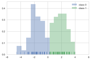
X0 = sp.stats.norm(-2, 1).rvs(40)
X1 = sp.stats.norm(+2, 1).rvs(60)
X = np.hstack([X0, X1])[:, np.newaxis]
y0 = np.zeros(40)
y1 = np.ones(60)
y = np.hstack([y0, y1])
sns.distplot(X0, rug=True, kde=False, norm_hist=True, label="class 0")
sns.distplot(X1, rug=True, kde=False, norm_hist=True, label="class 1")
plt.legend()
plt.xlim(-6,6)
plt.show()
#img 048-002-001
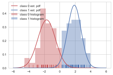
 from sklearn.naive_bayes import GaussianNB
clf_norm = GaussianNB().fit(X, y)
clf_norm.classes_
% array([0., 1.])
clf_norm.class_count_
% array([40., 60.])
clf_norm.class_prior_
% array([0.4, 0.6])
clf_norm.theta_, clf_norm.sigma_
% (array([[-1.68745753],
% [ 1.89131838]]), array([[1.13280656],
% [0.8668681 ]]))
xx = np.linspace(-6, 6, 100)
p0 = sp.stats.norm(clf_norm.theta_[0], clf_norm.sigma_[0]).pdf(xx)
p1 = sp.stats.norm(clf_norm.theta_[1], clf_norm.sigma_[1]).pdf(xx)
sns.distplot(X0, rug=True, kde=False, norm_hist=True, color="r", label="class 0 histogram")
sns.distplot(X1, rug=True, kde=False, norm_hist=True, color="b", label="class 1 histogram")
plt.plot(xx, p0, c="r", label="class 0 est. pdf")
plt.plot(xx, p1, c="b", label="class 1 est. pdf")
plt.legend()
plt.show()
#img 048-002-002
from sklearn.naive_bayes import GaussianNB
clf_norm = GaussianNB().fit(X, y)
clf_norm.classes_
% array([0., 1.])
clf_norm.class_count_
% array([40., 60.])
clf_norm.class_prior_
% array([0.4, 0.6])
clf_norm.theta_, clf_norm.sigma_
% (array([[-1.68745753],
% [ 1.89131838]]), array([[1.13280656],
% [0.8668681 ]]))
xx = np.linspace(-6, 6, 100)
p0 = sp.stats.norm(clf_norm.theta_[0], clf_norm.sigma_[0]).pdf(xx)
p1 = sp.stats.norm(clf_norm.theta_[1], clf_norm.sigma_[1]).pdf(xx)
sns.distplot(X0, rug=True, kde=False, norm_hist=True, color="r", label="class 0 histogram")
sns.distplot(X1, rug=True, kde=False, norm_hist=True, color="b", label="class 1 histogram")
plt.plot(xx, p0, c="r", label="class 0 est. pdf")
plt.plot(xx, p1, c="b", label="class 1 est. pdf")
plt.legend()
plt.show()
#img 048-002-002
 x_new = -1
clf_norm.predict_proba([[x_new]])
% array([[0.98327446, 0.01672554]])
px = sp.stats.norm(clf_norm.theta_, np.sqrt(clf_norm.sigma_)).pdf(x_new)
px
# array([[0.30425666],
# [0.00345028]])
p = px.flatten() * clf_norm.class_prior_
p
% array([0.12170266, 0.00207017])
clf_norm.class_prior_
% array([0.4, 0.6])
p / p.sum()
% array([0.98327446, 0.01672554])
Practice 1
Resolve iris classification question by using naive bayes classification model
and find following values
1. confusion matrix
1. classification report
1. ROC curve
1. AUC
@
using naive bayes classification model with bernoulli distribution
In bernoulli distribution, target variable y should have 0 or 1 but also independent variable x should have 0 or 1
You can do modeling about checking if specific words are contained in document by using bernoulli distribution
So you can apply bernoulli distribution model to building spam filtering
np.random.seed(0)
X = np.random.randint(2, size=(10, 4))
y = np.array([0,0,0,0,1,1,1,1,1,1])
print(X)
print(y)
% [[0 1 1 0]
% [1 1 1 1]
% [1 1 1 0]
% [0 1 0 0]
% [0 0 0 1]
% [0 1 1 0]
% [0 1 1 1]
% [1 0 1 0]
% [1 0 1 1]
% [0 1 1 0]]
% [0 0 0 0 1 1 1 1 1 1]
from sklearn.naive_bayes import BernoulliNB
clf_bern = BernoulliNB().fit(X, y)
clf_bern.classes_
% array([0, 1])
clf_bern.class_count_
% array([ 4., 6.])
np.exp(clf_bern.class_log_prior_)
% array([ 0.4, 0.6])
fc = clf_bern.feature_count_
fc
% array([[ 2., 4., 3., 1.],
% [ 2., 3., 5., 3.]])
fc / np.repeat(clf_bern.class_count_[:, np.newaxis], 4, axis=1)
% array([[ 0.5 , 1. , 0.75 , 0.25 ],
% [ 0.33333333, 0.5 , 0.83333333, 0.5 ]])
theta = np.exp(clf_bern.feature_log_prob_)
theta
% array([[ 0.5 , 0.83333333, 0.66666667, 0.33333333],
% [ 0.375 , 0.5 , 0.75 , 0.5 ]])
x_new = np.array([1, 1, 0, 0])
clf_bern.predict_proba([x_new])
% array([[ 0.72480181, 0.27519819]])
p = ((theta**x_new)*(1-theta)**(1-x_new)).prod(axis=1)*np.exp(clf_bern.class_log_prior_)
p / p.sum()
% array([ 0.72480181, 0.27519819])
x_new = np.array([0, 0, 1, 1])
clf_bern.predict_proba([x_new])
% array([[ 0.09530901, 0.90469099]])
p = ((theta**x_new)*(1-theta)**(1-x_new)).prod(axis=1)*np.exp(clf_bern.class_log_prior_)
p / p.sum()
% array([ 0.09530901, 0.90469099])
Practice 2
From NIST Digit classification question, you convert y value into 0 or 1 by using binarizer
and then you resolve question by using naive bayes classification model with bernoulli distribution
Additionally, resolve same question with arguments from binarizer by using BernoulliNB class
@
using naive bayes classification model with multinomial distribution
np.random.seed(0)
X0 = np.random.multinomial(10, [0.3, 0.5, 0.1, 0.1], size=4)
X1 = np.random.multinomial(8, [0.1, 0.1, 0.35, 0.45], size=6)
X = np.vstack([X0, X1])
y = np.array([0,0,0,0,1,1,1,1,1,1])
print(X)
print(y)
% [[3 4 1 2]
% [3 5 1 1]
% [3 3 0 4]
% [3 4 1 2]
% [1 2 1 4]
% [0 0 5 3]
% [1 2 4 1]
% [1 1 4 2]
% [0 1 2 5]
% [2 1 2 3]]
% [0 0 0 0 1 1 1 1 1 1]
from sklearn.naive_bayes import MultinomialNB
clf_mult = MultinomialNB().fit(X, y)
clf_mult.classes_
% array([0, 1])
clf_mult.class_count_
% array([ 4., 6.])
fc = clf_mult.feature_count_
fc
array([[ 12., 16., 3., 9.],
[ 5., 7., 18., 18.]])
fc / np.repeat(fc.sum(axis=1)[:, np.newaxis], 4, axis=1)
array([[ 0.3 , 0.4 , 0.075 , 0.225 ],
[ 0.10416667, 0.14583333, 0.375 , 0.375 ]])
clf_mult.alpha
% 1.0
(fc + clf_mult.alpha) / (np.repeat(fc.sum(axis=1)[:, np.newaxis], 4, axis=1) + clf_mult.alpha * X.shape[1])
% array([[ 0.29545455, 0.38636364, 0.09090909, 0.22727273],
% [ 0.11538462, 0.15384615, 0.36538462, 0.36538462]])
theta = np.exp(clf_mult.feature_log_prob_)
theta
% array([[ 0.29545455, 0.38636364, 0.09090909, 0.22727273],
% [ 0.11538462, 0.15384615, 0.36538462, 0.36538462]])
x_new = np.array([10, 10, 10, 10])
clf_mult.predict_proba([x_new])
% array([[ 0.38848858, 0.61151142]])
p = (theta**x_new).prod(axis=1)*np.exp(clf_bern.class_log_prior_)
p / p.sum()
% array([ 0.38848858, 0.61151142])
Practice 3
1. Resolve MNIST Digit classification question by using naive bayes classification model with multinomial distribution
1. Can you apply naive bayes classification model with multinomial distribution in case that x is real number not integer?
@
Let's try to apply naive bayes classification model to "20 News Group" data
import numpy as np
import scipy as sp
import pandas as pd
import statsmodels.api as sm
import statsmodels.formula.api as smf
import statsmodels.stats.api as sms
import sklearn as sk
import matplotlib as mpl
mpl.use('Agg')
import matplotlib.pylab as plt
from mpl_toolkits.mplot3d import Axes3D
import seaborn as sns
sns.set()
sns.set_style("whitegrid")
sns.set_color_codes()
%matplotlib inline
from sklearn.datasets import fetch_20newsgroups
news = fetch_20newsgroups(subset="all")
X = news.data
y = news.target
from sklearn.feature_extraction.text import TfidfVectorizer, HashingVectorizer, CountVectorizer
from sklearn.naive_bayes import MultinomialNB
from sklearn.pipeline import Pipeline
model1 = Pipeline([
('vect', CountVectorizer()),
('clf', MultinomialNB()),
])
model2 = Pipeline([
('vect', TfidfVectorizer()),
('clf', MultinomialNB()),
])
model3 = Pipeline([
('vect', TfidfVectorizer(stop_words="english")),
('clf', MultinomialNB()),
])
model4 = Pipeline([
('vect', TfidfVectorizer(stop_words="english",
token_pattern=r"\b[a-z0-9_\-\.]+[a-z][a-z0-9_\-\.]+\b")),
('clf', MultinomialNB()),
])
%%time
from sklearn.model_selection import cross_val_score, KFold
for i, clf in enumerate([model1, model2, model3, model4]):
scores = cross_val_score(clf, X, y, cv=5)
print(("Model{0:d}: Mean score: {1:.3f})").format(i, np.mean(scores)))
% Model0: Mean score: 0.855)
% Model1: Mean score: 0.856)
% Model2: Mean score: 0.883)
% Model3: Mean score: 0.888)
% Wall time: 2min 50s
Practice 4
How will you resolve question if x is composed of $x_{1}$ has real numbers, $x_{2}$ has 0 or 1, etc?
x_new = -1
clf_norm.predict_proba([[x_new]])
% array([[0.98327446, 0.01672554]])
px = sp.stats.norm(clf_norm.theta_, np.sqrt(clf_norm.sigma_)).pdf(x_new)
px
# array([[0.30425666],
# [0.00345028]])
p = px.flatten() * clf_norm.class_prior_
p
% array([0.12170266, 0.00207017])
clf_norm.class_prior_
% array([0.4, 0.6])
p / p.sum()
% array([0.98327446, 0.01672554])
Practice 1
Resolve iris classification question by using naive bayes classification model
and find following values
1. confusion matrix
1. classification report
1. ROC curve
1. AUC
@
using naive bayes classification model with bernoulli distribution
In bernoulli distribution, target variable y should have 0 or 1 but also independent variable x should have 0 or 1
You can do modeling about checking if specific words are contained in document by using bernoulli distribution
So you can apply bernoulli distribution model to building spam filtering
np.random.seed(0)
X = np.random.randint(2, size=(10, 4))
y = np.array([0,0,0,0,1,1,1,1,1,1])
print(X)
print(y)
% [[0 1 1 0]
% [1 1 1 1]
% [1 1 1 0]
% [0 1 0 0]
% [0 0 0 1]
% [0 1 1 0]
% [0 1 1 1]
% [1 0 1 0]
% [1 0 1 1]
% [0 1 1 0]]
% [0 0 0 0 1 1 1 1 1 1]
from sklearn.naive_bayes import BernoulliNB
clf_bern = BernoulliNB().fit(X, y)
clf_bern.classes_
% array([0, 1])
clf_bern.class_count_
% array([ 4., 6.])
np.exp(clf_bern.class_log_prior_)
% array([ 0.4, 0.6])
fc = clf_bern.feature_count_
fc
% array([[ 2., 4., 3., 1.],
% [ 2., 3., 5., 3.]])
fc / np.repeat(clf_bern.class_count_[:, np.newaxis], 4, axis=1)
% array([[ 0.5 , 1. , 0.75 , 0.25 ],
% [ 0.33333333, 0.5 , 0.83333333, 0.5 ]])
theta = np.exp(clf_bern.feature_log_prob_)
theta
% array([[ 0.5 , 0.83333333, 0.66666667, 0.33333333],
% [ 0.375 , 0.5 , 0.75 , 0.5 ]])
x_new = np.array([1, 1, 0, 0])
clf_bern.predict_proba([x_new])
% array([[ 0.72480181, 0.27519819]])
p = ((theta**x_new)*(1-theta)**(1-x_new)).prod(axis=1)*np.exp(clf_bern.class_log_prior_)
p / p.sum()
% array([ 0.72480181, 0.27519819])
x_new = np.array([0, 0, 1, 1])
clf_bern.predict_proba([x_new])
% array([[ 0.09530901, 0.90469099]])
p = ((theta**x_new)*(1-theta)**(1-x_new)).prod(axis=1)*np.exp(clf_bern.class_log_prior_)
p / p.sum()
% array([ 0.09530901, 0.90469099])
Practice 2
From NIST Digit classification question, you convert y value into 0 or 1 by using binarizer
and then you resolve question by using naive bayes classification model with bernoulli distribution
Additionally, resolve same question with arguments from binarizer by using BernoulliNB class
@
using naive bayes classification model with multinomial distribution
np.random.seed(0)
X0 = np.random.multinomial(10, [0.3, 0.5, 0.1, 0.1], size=4)
X1 = np.random.multinomial(8, [0.1, 0.1, 0.35, 0.45], size=6)
X = np.vstack([X0, X1])
y = np.array([0,0,0,0,1,1,1,1,1,1])
print(X)
print(y)
% [[3 4 1 2]
% [3 5 1 1]
% [3 3 0 4]
% [3 4 1 2]
% [1 2 1 4]
% [0 0 5 3]
% [1 2 4 1]
% [1 1 4 2]
% [0 1 2 5]
% [2 1 2 3]]
% [0 0 0 0 1 1 1 1 1 1]
from sklearn.naive_bayes import MultinomialNB
clf_mult = MultinomialNB().fit(X, y)
clf_mult.classes_
% array([0, 1])
clf_mult.class_count_
% array([ 4., 6.])
fc = clf_mult.feature_count_
fc
array([[ 12., 16., 3., 9.],
[ 5., 7., 18., 18.]])
fc / np.repeat(fc.sum(axis=1)[:, np.newaxis], 4, axis=1)
array([[ 0.3 , 0.4 , 0.075 , 0.225 ],
[ 0.10416667, 0.14583333, 0.375 , 0.375 ]])
clf_mult.alpha
% 1.0
(fc + clf_mult.alpha) / (np.repeat(fc.sum(axis=1)[:, np.newaxis], 4, axis=1) + clf_mult.alpha * X.shape[1])
% array([[ 0.29545455, 0.38636364, 0.09090909, 0.22727273],
% [ 0.11538462, 0.15384615, 0.36538462, 0.36538462]])
theta = np.exp(clf_mult.feature_log_prob_)
theta
% array([[ 0.29545455, 0.38636364, 0.09090909, 0.22727273],
% [ 0.11538462, 0.15384615, 0.36538462, 0.36538462]])
x_new = np.array([10, 10, 10, 10])
clf_mult.predict_proba([x_new])
% array([[ 0.38848858, 0.61151142]])
p = (theta**x_new).prod(axis=1)*np.exp(clf_bern.class_log_prior_)
p / p.sum()
% array([ 0.38848858, 0.61151142])
Practice 3
1. Resolve MNIST Digit classification question by using naive bayes classification model with multinomial distribution
1. Can you apply naive bayes classification model with multinomial distribution in case that x is real number not integer?
@
Let's try to apply naive bayes classification model to "20 News Group" data
import numpy as np
import scipy as sp
import pandas as pd
import statsmodels.api as sm
import statsmodels.formula.api as smf
import statsmodels.stats.api as sms
import sklearn as sk
import matplotlib as mpl
mpl.use('Agg')
import matplotlib.pylab as plt
from mpl_toolkits.mplot3d import Axes3D
import seaborn as sns
sns.set()
sns.set_style("whitegrid")
sns.set_color_codes()
%matplotlib inline
from sklearn.datasets import fetch_20newsgroups
news = fetch_20newsgroups(subset="all")
X = news.data
y = news.target
from sklearn.feature_extraction.text import TfidfVectorizer, HashingVectorizer, CountVectorizer
from sklearn.naive_bayes import MultinomialNB
from sklearn.pipeline import Pipeline
model1 = Pipeline([
('vect', CountVectorizer()),
('clf', MultinomialNB()),
])
model2 = Pipeline([
('vect', TfidfVectorizer()),
('clf', MultinomialNB()),
])
model3 = Pipeline([
('vect', TfidfVectorizer(stop_words="english")),
('clf', MultinomialNB()),
])
model4 = Pipeline([
('vect', TfidfVectorizer(stop_words="english",
token_pattern=r"\b[a-z0-9_\-\.]+[a-z][a-z0-9_\-\.]+\b")),
('clf', MultinomialNB()),
])
%%time
from sklearn.model_selection import cross_val_score, KFold
for i, clf in enumerate([model1, model2, model3, model4]):
scores = cross_val_score(clf, X, y, cv=5)
print(("Model{0:d}: Mean score: {1:.3f})").format(i, np.mean(scores)))
% Model0: Mean score: 0.855)
% Model1: Mean score: 0.856)
% Model2: Mean score: 0.883)
% Model3: Mean score: 0.888)
% Wall time: 2min 50s
Practice 4
How will you resolve question if x is composed of $x_{1}$ has real numbers, $x_{2}$ has 0 or 1, etc?