================================================================================
- Keywords
Discrete random variable
Cumulitive distribution function
Probability mass function
Probability density function
Univariate gaussian probability density function
Multivariate gaussian probability density function
Covariance
================================================================================
Univariate Gaussian probability density function.
# When you use discrete random variable
discrete_values=discrete_random_variable(result_from_trials)
prob_values=cumulitive_distribution_func(discrete_values)
probability_mass_func=defferentiation(cumulitive_distribution_func)
# When you use continuous random variable
continuous_values=continuous_random_variable(result_from_trials)
prob_values=cumulitive_distribution_func(continuous_values)
probability_density_func=defferentiation(cumulitive_distribution_func)
================================================================================
When you deal with continuous random variable in your statistical project,
how can you give values to other people?
continuous_values=continuous_random_variable(result_from_trials)
continuous_prob_vals=probability_density_func(continuous_values)
$$$-\infty<$$$ continuous_prob_vals $$$< \infty$$$
================================================================================
* Question: how can you hand in continuous_prob_vals to other people
because it's too many?
* You actually can't do it.
* You should hand in "equation" to other people, which can generate continuous_prob_vals
* Predefined equations are like Gaussian normal distribution, bernoulli distribution, dirichlet distribution, etc
================================================================================
* Functions which can represent "probability density or probability distribution" can have various and arbitrary shapes.
* But practically, in real world problems, many cases have pattern-based probability distribution like this
 ================================================================================
* How can you express those graphs into a math formula?
* Math formulas which can represent above graphs are created by mathematicians.
================================================================================
* Math formular for "univariate Gaussian probability density function"
* $$$f_X(x)=\frac{1}{\sqrt{2\pi}\sigma}\exp \left[ -\frac{1}{2} \left( \frac{X-\mu}{\sigma} \right)^2 \right]$$$
* $$$f_X(x)$$$: function f is function wrt univariate random variable X
numbers=random_variable_X(x)
* $$$\sigma$$$: standard deviation ($$$\sigma^2$$$ is variance)
* $$$\mu$$$: expectation value, average
* $$$e$$$: 2.146...
================================================================================
* Simple notation for Gaussian probability density function
$$$f(x;\mu=0,\sigma^2=4)$$$
* Formula notation for Gaussian probability density function
$$$\frac{1}{\sqrt{2\pi}2}\exp \left[ -\frac{1}{2} \left( \frac{X-0}{2} \right)^2 \right]$$$
================================================================================
"Univariate Gaussian probability density function" has one random variable X like this
See x axis. It can have one value at a time like $$$x=-5, -4, \cdots$$$
-5=random_variable_X(result1)
-4=random_variable_X(result2)
================================================================================
* How can you express those graphs into a math formula?
* Math formulas which can represent above graphs are created by mathematicians.
================================================================================
* Math formular for "univariate Gaussian probability density function"
* $$$f_X(x)=\frac{1}{\sqrt{2\pi}\sigma}\exp \left[ -\frac{1}{2} \left( \frac{X-\mu}{\sigma} \right)^2 \right]$$$
* $$$f_X(x)$$$: function f is function wrt univariate random variable X
numbers=random_variable_X(x)
* $$$\sigma$$$: standard deviation ($$$\sigma^2$$$ is variance)
* $$$\mu$$$: expectation value, average
* $$$e$$$: 2.146...
================================================================================
* Simple notation for Gaussian probability density function
$$$f(x;\mu=0,\sigma^2=4)$$$
* Formula notation for Gaussian probability density function
$$$\frac{1}{\sqrt{2\pi}2}\exp \left[ -\frac{1}{2} \left( \frac{X-0}{2} \right)^2 \right]$$$
================================================================================
"Univariate Gaussian probability density function" has one random variable X like this
See x axis. It can have one value at a time like $$$x=-5, -4, \cdots$$$
-5=random_variable_X(result1)
-4=random_variable_X(result2)
 ================================================================================
* "Multivariate Gaussian probability density function"
$$$f_X(x)=\dfrac{1}{(2\pi)^{\frac{n}{2}}\sqrt{|\Sigma|}} \exp \left[ -\frac{1}{2} (x-\mu)^T\Sigma^{-1}(x-\mu) \right]$$$
* $$$n$$$: dimension of vectors
================================================================================
$$$X=\begin{bmatrix} x_1\\x_2\\\vdots\\x_N \end{bmatrix}$$$
If $$$n=2$$$, X can have 2 random variables like height=170, weight=60 at a time.
170=random_variable_1(result_from_measuring_height)
60=random_variable_2(result_from_measuring_weight)
================================================================================
$$$\mu=\begin{bmatrix} \mu_1\\\mu_2\\\vdots\\\mu_N \end{bmatrix}$$$
$$$\mu_1$$$: Average from random variable 1
$$$\vdots$$$
$$$\mu_N$$$: Average from random variable N
If $$$n=2$$$ like height and weight,
and suppose you extract height and weight data from 10 people.
$$$\mu_1$$$: average of 10 heights
$$$\mu_2$$$: average of 10 weights
* Code
height_val1=random_variable_1(measured_height1)
...
height_val10=random_variable_1(measured_height10)
mu_1=mean([height_val1,...,height_val10])
weight_val1=random_variable_2(measured_weight1)
...
weight_val10=random_variable_2(measured_weight10)
mu_2s=mean([weight_val1,...,weight_val10])
================================================================================
When you use univariate ramdom variable, you use variance
(actually you use std $$$\sigma$$$ from $$$\sqrt{\sigma^2}$$$).
* Code
height_val1=random_variable_1(measured_height1)
...
height_val10=random_variable_1(measured_height10)
variance_val_of_RV1=variance_func([height_val1,...,height_val10])
================================================================================
But when you use multivariate ramdom variable, you use covariance $$$\Sigma$$$.
$$$\Sigma=\begin{bmatrix}
\sigma_1^2 & & & \\
& \sigma_2^2 & & \\
& & \ddots & \\
& & & \sigma_N^2
\end{bmatrix}$$$
$$$\sigma_1^2$$$: variance of random variable 1
$$$\vdots$$$
$$$\sigma_N^2$$$: variance of random variable N
Elements in off-diagonal regions: covariance values between random variables
================================================================================
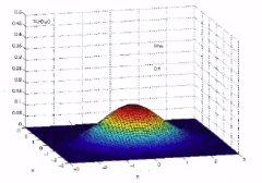
When $$$n=2$$$, for example,
when you have 2 random variables like random_variable1 for body_weight, random_variable2 for body_height
multivariate Gaussian probability distribution function shapes like this
================================================================================
* "Multivariate Gaussian probability density function"
$$$f_X(x)=\dfrac{1}{(2\pi)^{\frac{n}{2}}\sqrt{|\Sigma|}} \exp \left[ -\frac{1}{2} (x-\mu)^T\Sigma^{-1}(x-\mu) \right]$$$
* $$$n$$$: dimension of vectors
================================================================================
$$$X=\begin{bmatrix} x_1\\x_2\\\vdots\\x_N \end{bmatrix}$$$
If $$$n=2$$$, X can have 2 random variables like height=170, weight=60 at a time.
170=random_variable_1(result_from_measuring_height)
60=random_variable_2(result_from_measuring_weight)
================================================================================
$$$\mu=\begin{bmatrix} \mu_1\\\mu_2\\\vdots\\\mu_N \end{bmatrix}$$$
$$$\mu_1$$$: Average from random variable 1
$$$\vdots$$$
$$$\mu_N$$$: Average from random variable N
If $$$n=2$$$ like height and weight,
and suppose you extract height and weight data from 10 people.
$$$\mu_1$$$: average of 10 heights
$$$\mu_2$$$: average of 10 weights
* Code
height_val1=random_variable_1(measured_height1)
...
height_val10=random_variable_1(measured_height10)
mu_1=mean([height_val1,...,height_val10])
weight_val1=random_variable_2(measured_weight1)
...
weight_val10=random_variable_2(measured_weight10)
mu_2s=mean([weight_val1,...,weight_val10])
================================================================================
When you use univariate ramdom variable, you use variance
(actually you use std $$$\sigma$$$ from $$$\sqrt{\sigma^2}$$$).
* Code
height_val1=random_variable_1(measured_height1)
...
height_val10=random_variable_1(measured_height10)
variance_val_of_RV1=variance_func([height_val1,...,height_val10])
================================================================================
But when you use multivariate ramdom variable, you use covariance $$$\Sigma$$$.
$$$\Sigma=\begin{bmatrix}
\sigma_1^2 & & & \\
& \sigma_2^2 & & \\
& & \ddots & \\
& & & \sigma_N^2
\end{bmatrix}$$$
$$$\sigma_1^2$$$: variance of random variable 1
$$$\vdots$$$
$$$\sigma_N^2$$$: variance of random variable N
Elements in off-diagonal regions: covariance values between random variables
================================================================================
When $$$n=2$$$, for example,
when you have 2 random variables like random_variable1 for body_weight, random_variable2 for body_height
multivariate Gaussian probability distribution function shapes like this
 ================================================================================
Simple notation
$$$f(\begin{bmatrix} x_1\\x_2 \end{bmatrix};\mu=\begin{bmatrix} 1\\2 \end{bmatrix},\Sigma=\begin{bmatrix} 2&&0\\0&&4 \end{bmatrix})$$$
Formula notation
$$$\frac{1}{\sqrt{(2\pi)^2}\sqrt{8}}\exp \left[ -\frac{1}{2} \begin{bmatrix} x_1-1&&x_2-2 \end{bmatrix} \begin{bmatrix} 0.5&&0\\0&&0.25 \end{bmatrix} \begin{bmatrix} x_1-1\\x_2-2 \end{bmatrix} \right]$$$
================================================================================
Simple notation
$$$f(\begin{bmatrix} x_1\\x_2 \end{bmatrix};\mu=\begin{bmatrix} 1\\2 \end{bmatrix},\Sigma=\begin{bmatrix} 2&&0\\0&&4 \end{bmatrix})$$$
Formula notation
$$$\frac{1}{\sqrt{(2\pi)^2}\sqrt{8}}\exp \left[ -\frac{1}{2} \begin{bmatrix} x_1-1&&x_2-2 \end{bmatrix} \begin{bmatrix} 0.5&&0\\0&&0.25 \end{bmatrix} \begin{bmatrix} x_1-1\\x_2-2 \end{bmatrix} \right]$$$