================================================================================
When you classify 2 products (one is expensive, one is cheap),
if your classifier classifies expensive one to cheap one, customer doesn't make a complain.
But if your classifier classifies cheap one to expensive one, customer will make a complain.
================================================================================
That is, you should consider this scenario
where cost happens when classifier makes mis-classification.
================================================================================
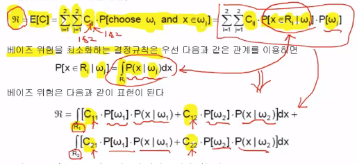
Let's call cost as $$$C_{ij}$$$
$$$\text{Final Cost} \\
= E[C] \\$$$
* $$$E[C]$$$: expectation value of cost C
$$$= \sum\limits_{i=1}^{2} \sum\limits_{j=1}^{2} C_{ij} \cdot P[\text{choose }\omega_i \text{ and } x\in \omega_j] \\$$$
* $$$C_{ij}$$$: cost value when classifier missclassifies $$$\omega_j$$$ to $$$\omega_i$$$
* $$$P[\text{choose }\omega_i \text{ and } x\in \omega_j]$$$: Probability of missclassification occuring
$$$= \sum\limits_{i=1}^{2} \sum\limits_{j=1}^{2} C_{ij} \cdot P[x\in R_i|\omega_j] \cdot P[\omega_j]$$$
* Use Bayes rule: posterior probability = likelihood $$$\times$$$ prior probablity
================================================================================
* Precondition:
$$$P[x\in R_i|\omega_j] = \int_{R_i} P(x|\omega_j) dx$$$
* $$$P[x\in R_i|\omega_j]$$$: probability of x is in R_i, when $$$\omega_j$$$ is given
* $$$\int_{R_i} P(x|\omega_j)$$$: perform integrate likelihood in $$$R_i$$$
================================================================================
By using above precondition,
you can write Bayes error into
 ================================================================================
* Likelihood is expressed as follow
================================================================================
* Likelihood is expressed as follow
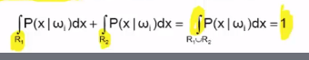 * Summed area should be 1
 ================================================================================
Conclusion of this lecture:
================================================================================
Conclusion of this lecture:
 * If you consider cost terms when using LRT,
you can get classifier (or decision boundary) which can minimize Bayes risk
================================================================================
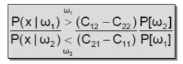
$$$\dfrac{P(x|\omega_1)}{P(x|\omega_2)} \;\; \dfrac{\overset{\omega_1}{>}}{\overset{<}{\omega_2}} \;\; \dfrac{(C_{12}-C_{22})P[\omega_2]}{(C_{21}-C_{11})P[\omega_1]}$$$
If likelihood ratio of $$$\omega_1$$$ and $$$\omega_2$$$ is greater than $$$\frac{\text{prior probablity of }\omega_1}{\text{prior probablity of }\omega_2}$$$
you choose $$$\omega_1$$$
If likelihood ratio of $$$\omega_1$$$ and $$$\omega_2$$$ is less than $$$\frac{\text{prior probablity of }\omega_1}{\text{prior probablity of }\omega_2}$$$
you choose $$$\omega_2$$$
Above one is LRT decision rule.
But cost constant term is added onto it.
Then, it becomes decision boundary which minimizes Bayes risk
================================================================================
Example
* If you consider cost terms when using LRT,
you can get classifier (or decision boundary) which can minimize Bayes risk
================================================================================
$$$\dfrac{P(x|\omega_1)}{P(x|\omega_2)} \;\; \dfrac{\overset{\omega_1}{>}}{\overset{<}{\omega_2}} \;\; \dfrac{(C_{12}-C_{22})P[\omega_2]}{(C_{21}-C_{11})P[\omega_1]}$$$
If likelihood ratio of $$$\omega_1$$$ and $$$\omega_2$$$ is greater than $$$\frac{\text{prior probablity of }\omega_1}{\text{prior probablity of }\omega_2}$$$
you choose $$$\omega_1$$$
If likelihood ratio of $$$\omega_1$$$ and $$$\omega_2$$$ is less than $$$\frac{\text{prior probablity of }\omega_1}{\text{prior probablity of }\omega_2}$$$
you choose $$$\omega_2$$$
Above one is LRT decision rule.
But cost constant term is added onto it.
Then, it becomes decision boundary which minimizes Bayes risk
================================================================================
Example
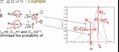 Red line: likelihood probability density function of class $$$\omega_1$$$
Blue line: likelihood probability density function of class $$$\omega_2$$$
$$$0$$$: mean value of class $$$\omega_1$$$
$$$2$$$: mean value of class $$$\omega_2$$$
$$$\sqrt{3}$$$: variance of class $$$\omega_1$$$
$$$1$$$: variance of class $$$\omega_2$$$
================================================================================
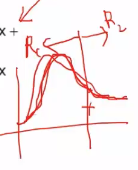
You can think of optimal decision boundary intuitively
which separates feature space
Red line: likelihood probability density function of class $$$\omega_1$$$
Blue line: likelihood probability density function of class $$$\omega_2$$$
$$$0$$$: mean value of class $$$\omega_1$$$
$$$2$$$: mean value of class $$$\omega_2$$$
$$$\sqrt{3}$$$: variance of class $$$\omega_1$$$
$$$1$$$: variance of class $$$\omega_2$$$
================================================================================
You can think of optimal decision boundary intuitively
which separates feature space
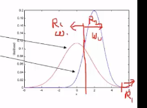 $$$\omega_1$$$: class 1
$$$\omega_2$$$: class 2
$$$R_1$$$: region of class $$$\omega_1$$$
$$$R_2$$$: region of class $$$\omega_2$$$
================================================================================
Suppose prior probability is same: $$$P[\omega_1]=P[\omega_2]=0.5$$$
$$$C_{11}=C_{22}=0$$$: classify class 1 to class 1, classify class 2 to class 2, then, costs are 0
$$$C_{12}=1$$$: misclassify class 1 to class 2, then, its cost is 1
$$$C_{21}=\sqrt{3}$$$: misclassify class 2 to class 1, then, its cost is $$$\sqrt{3}$$$
================================================================================
Put values into following equation
$$$\dfrac{P(x|\omega_1)}{P(x|\omega_2)} \;\; \dfrac{\overset{\omega_1}{>}}{\overset{<}{\omega_2}} \;\; \dfrac{(C_{12}-C_{22})P[\omega_2]}{(C_{21}-C_{11})P[\omega_1]}$$$
$$$P(x|\omega_1)=\frac{1}{\sqrt{2\pi}\sqrt{3}} e^{-\frac{1}{2}\times \frac{x^2}{3}}$$$
$$$P(x|\omega_2)=\frac{1}{\sqrt{2\pi}} e^{-\frac{1}{2}\times (x-2)^2}$$$
$$$\dfrac{\frac{1}{\sqrt{2\pi}\sqrt{3}} e^{-\frac{1}{2}\times \frac{x^2}{3}}}{\frac{1}{\sqrt{2\pi}} e^{-\frac{1}{2}\times (x-2)^2}} \;\; \dfrac{\overset{\omega_1}{>}}{\overset{<}{\omega_2}} \;\; \dfrac{1}{\sqrt{3}} $$$
Simplify above equation, then, you get:
$$$2x^2-12x+12 \;\; \frac{\text{if } > \text{ then you choose } \omega_1}{\text{if } < \text{ then you choose } \omega_2} \;\; 0 $$$
Finally, you can get $$$x=4.73, 1.27$$$ which is decision boundary minimizing Bayes risk
$$$\omega_1$$$: class 1
$$$\omega_2$$$: class 2
$$$R_1$$$: region of class $$$\omega_1$$$
$$$R_2$$$: region of class $$$\omega_2$$$
================================================================================
Suppose prior probability is same: $$$P[\omega_1]=P[\omega_2]=0.5$$$
$$$C_{11}=C_{22}=0$$$: classify class 1 to class 1, classify class 2 to class 2, then, costs are 0
$$$C_{12}=1$$$: misclassify class 1 to class 2, then, its cost is 1
$$$C_{21}=\sqrt{3}$$$: misclassify class 2 to class 1, then, its cost is $$$\sqrt{3}$$$
================================================================================
Put values into following equation
$$$\dfrac{P(x|\omega_1)}{P(x|\omega_2)} \;\; \dfrac{\overset{\omega_1}{>}}{\overset{<}{\omega_2}} \;\; \dfrac{(C_{12}-C_{22})P[\omega_2]}{(C_{21}-C_{11})P[\omega_1]}$$$
$$$P(x|\omega_1)=\frac{1}{\sqrt{2\pi}\sqrt{3}} e^{-\frac{1}{2}\times \frac{x^2}{3}}$$$
$$$P(x|\omega_2)=\frac{1}{\sqrt{2\pi}} e^{-\frac{1}{2}\times (x-2)^2}$$$
$$$\dfrac{\frac{1}{\sqrt{2\pi}\sqrt{3}} e^{-\frac{1}{2}\times \frac{x^2}{3}}}{\frac{1}{\sqrt{2\pi}} e^{-\frac{1}{2}\times (x-2)^2}} \;\; \dfrac{\overset{\omega_1}{>}}{\overset{<}{\omega_2}} \;\; \dfrac{1}{\sqrt{3}} $$$
Simplify above equation, then, you get:
$$$2x^2-12x+12 \;\; \frac{\text{if } > \text{ then you choose } \omega_1}{\text{if } < \text{ then you choose } \omega_2} \;\; 0 $$$
Finally, you can get $$$x=4.73, 1.27$$$ which is decision boundary minimizing Bayes risk
 ================================================================================