================================================================================
In previous lectures, you learned "how to estimate probability density function of population
using parameters of samples from population"
================================================================================
Now, you will not suppose "probability density function" as Gaussian distribution shape
You will suppose arbitrary shape.
Then, you can't use parameters to estimate PDF
================================================================================
Likelihood: density of each class, $$$p(x|\omega_i)$$$
Previous chapters:
1. You supposed you know likelihood which is PDF of specific class (you used MLE)
2. You supposed you know parametric shape of likelihood (parametric estimation)
================================================================================
* You won't suppose the shape of PDF
* You will estimate PDF via sample
================================================================================
* Non parametric PDF estimation
- Histogram
- Kernel density estimation
- k-NNR
================================================================================
Sample data
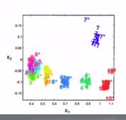 Population data's PDF which is composed of multiples classes
 PDF: $$$P(x_1,x_2|\omega_i)$$$
================================================================================
* Histogram
* It decribes density of data
* You separate data by fixed intervals
* You count frequency of data in each interval
* High frequency -> Tall vertical bar
PDF: $$$P(x_1,x_2|\omega_i)$$$
================================================================================
* Histogram
* It decribes density of data
* You separate data by fixed intervals
* You count frequency of data in each interval
* High frequency -> Tall vertical bar
 ================================================================================
* To get probability value, you can use following
$$$P_{H}(x) = \frac{1}{N} \frac{\text{height of bin}}{\text{width of bin}}$$$
* Advantage:
- Easy to write
* Disadvantage:
- Final shape from density estimation depends on "starting position of the bins"
- Density can look "not continous"
But it's not actuallly "discontinuity", it just look "discontinuity" due to interval of bin
- Curse of dimention: more dimension creates more number of bins
Then, most of bins become empty, resulting "discontinuity-like looking"
- So, Histogram is not useful for practical analysis
but it's useful for rapid visualization
================================================================================
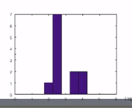
* Example
12 data:
2.1, 2.4, 2.3, 2.4, 2.47, 2.7, 2.6, 2.65, 3.3, 3.39, 3.8, 3.87
* Find Histogram
- width of big: 0.5
- Interval: 1.0 - 1.5, 2.0 - 2.5, ...
* Code
Y=[2.1, 2.4, 2.3, 2.4, 2.47, 2.7, 2.6, 2.65, 3.3, 3.39, 3.8, 3.87]
X=[0.25:0.5:5]
N=HIST(Y,X)
================================================================================
* To get probability value, you can use following
$$$P_{H}(x) = \frac{1}{N} \frac{\text{height of bin}}{\text{width of bin}}$$$
* Advantage:
- Easy to write
* Disadvantage:
- Final shape from density estimation depends on "starting position of the bins"
- Density can look "not continous"
But it's not actuallly "discontinuity", it just look "discontinuity" due to interval of bin
- Curse of dimention: more dimension creates more number of bins
Then, most of bins become empty, resulting "discontinuity-like looking"
- So, Histogram is not useful for practical analysis
but it's useful for rapid visualization
================================================================================
* Example
12 data:
2.1, 2.4, 2.3, 2.4, 2.47, 2.7, 2.6, 2.65, 3.3, 3.39, 3.8, 3.87
* Find Histogram
- width of big: 0.5
- Interval: 1.0 - 1.5, 2.0 - 2.5, ...
* Code
Y=[2.1, 2.4, 2.3, 2.4, 2.47, 2.7, 2.6, 2.65, 3.3, 3.39, 3.8, 3.87]
X=[0.25:0.5:5]
N=HIST(Y,X)
 Y=[2.1, 2.4, 2.3, 2.4, 2.47, 2.7, 2.6, 2.65, 3.3, 3.39, 3.8, 3.87]
X=[0.5:0.5:5]
N=HIST(Y,X)
Y=[2.1, 2.4, 2.3, 2.4, 2.47, 2.7, 2.6, 2.65, 3.3, 3.39, 3.8, 3.87]
X=[0.5:0.5:5]
N=HIST(Y,X)
 ================================================================================