12-01 Dimentionality reduction by PCA(principle component analysis)
@
12-06 Dimentionality reduction by PCA(principle component analysis)
=========================================================
Limitation 1 of PCA
=========================================================
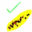
Since PCA uses eigenvector of covariance matrix, PCA can be used to find independent axis on data which follows unimodal gaussian
That is, PCA is hardly able to used for case where data doesn't follow gaussian or follows nonlinear multimodal pattern
unimodal : variance of data is concentrated on one side
gaussian : density is highest on center
2018-06-06 07-52-05.png
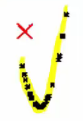
 Nonlinear : data is scattered here and there
2018-06-06 07-51-54.png
Nonlinear : data is scattered here and there
2018-06-06 07-51-54.png
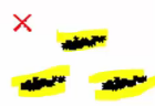
 multimodal pattern
2018-06-06 07-51-41.png
multimodal pattern
2018-06-06 07-51-41.png
 =========================================================
Limitation 2 of PCA
=========================================================
Since PCA doesn't consider class label, PCA doesn't consider distinguishability of classes
In other words, PCA sees data as one chuck of data (data involved in one class), not as data composed of various classes
But remember purpose of PCA is to reduce dimensionality with keeping characteristic of original data
PCA is all about changing axis which will be used for projection
Direction of axis is most important when using PCA
In other words, you can say you perform "coordinate rotation" to make direction of axis matched with direction of largest variance
=========================================================
history of PCA
=========================================================
PCA is matured technique in multivariate analysis domain
PCA is also known as Karhunen-Loeve transform (KL-transform) in IT communication domain
KL-transform is multivariate data processing method which reduces dimensionality
where data is located in, with keeping characteristic of data in high dimensionality
KL-transform is needed because when performing communication the smaller size of data is the better efficiency becomes
KL-transform was introduced by Loeve in 1963
After fixing KL-transform several times, PCA was introduced by Pearson in 1901
=========================================================
Example
=========================================================
You can see data plotted in 3 dimension variance plot
Data follows gaussian distribution
When dealing with data following gaussian distribution,
you need to know parameters of data (average, covariance matrix in case of multidimension data, etc)
2018-06-06 08-18-55.png
=========================================================
Limitation 2 of PCA
=========================================================
Since PCA doesn't consider class label, PCA doesn't consider distinguishability of classes
In other words, PCA sees data as one chuck of data (data involved in one class), not as data composed of various classes
But remember purpose of PCA is to reduce dimensionality with keeping characteristic of original data
PCA is all about changing axis which will be used for projection
Direction of axis is most important when using PCA
In other words, you can say you perform "coordinate rotation" to make direction of axis matched with direction of largest variance
=========================================================
history of PCA
=========================================================
PCA is matured technique in multivariate analysis domain
PCA is also known as Karhunen-Loeve transform (KL-transform) in IT communication domain
KL-transform is multivariate data processing method which reduces dimensionality
where data is located in, with keeping characteristic of data in high dimensionality
KL-transform is needed because when performing communication the smaller size of data is the better efficiency becomes
KL-transform was introduced by Loeve in 1963
After fixing KL-transform several times, PCA was introduced by Pearson in 1901
=========================================================
Example
=========================================================
You can see data plotted in 3 dimension variance plot
Data follows gaussian distribution
When dealing with data following gaussian distribution,
you need to know parameters of data (average, covariance matrix in case of multidimension data, etc)
2018-06-06 08-18-55.png
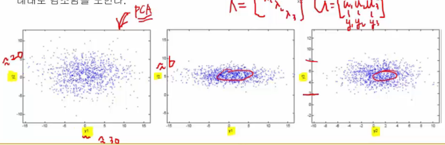
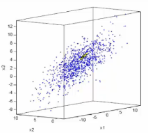 Parameters of data which follows 3 dimension gaussian distribution :
average vector $$$\mu=\begin{bmatrix} 0\\5\\2 \end{bmatrix}$$$
covariance matrix $$$\Sigma=\begin{bmatrix} 25&-1&7\\-1&4&-4\\7&-4&10 \end{bmatrix}$$$
As you can see, data isn't lined up with specific one axis
Step:
1. You find covariance matrix $$$\Sigma$$$
2. You find $$$U\Lambda U^{-1}$$$ (eigenvalue $$$\Lambda$$$, eigenvector U) by using eigen() in matlab
Concise shape of U and $$$\Lambda$$$ :
3by3 matrix containing 3 eigenvalues $$$\Lambda = \begin{bmatrix} \lambda_{1}&x&x \\ x&\lambda_{2}&x \\ x&x&\lambda_{3} \end{bmatrix}$$$
3 eigenvectors contained by U matrix as column vector, $$$U = \begin{bmatrix} x&u_{1}&x \\ x&u_{2}&x \\ x&u_{3}&x \end{bmatrix}$$$
=========================================================
let's reduce 3 dimensional vector to 2 dimensional vector
=========================================================
2018-06-06 08-34-57.png
Parameters of data which follows 3 dimension gaussian distribution :
average vector $$$\mu=\begin{bmatrix} 0\\5\\2 \end{bmatrix}$$$
covariance matrix $$$\Sigma=\begin{bmatrix} 25&-1&7\\-1&4&-4\\7&-4&10 \end{bmatrix}$$$
As you can see, data isn't lined up with specific one axis
Step:
1. You find covariance matrix $$$\Sigma$$$
2. You find $$$U\Lambda U^{-1}$$$ (eigenvalue $$$\Lambda$$$, eigenvector U) by using eigen() in matlab
Concise shape of U and $$$\Lambda$$$ :
3by3 matrix containing 3 eigenvalues $$$\Lambda = \begin{bmatrix} \lambda_{1}&x&x \\ x&\lambda_{2}&x \\ x&x&\lambda_{3} \end{bmatrix}$$$
3 eigenvectors contained by U matrix as column vector, $$$U = \begin{bmatrix} x&u_{1}&x \\ x&u_{2}&x \\ x&u_{3}&x \end{bmatrix}$$$
=========================================================
let's reduce 3 dimensional vector to 2 dimensional vector
=========================================================
2018-06-06 08-34-57.png
 =========================================================
Example
=========================================================
그림은 3차원 자료 3D 펭귄모양을 2차원으로 projecion 한 것이다.
처음의 projecion 에서는 모양이 잘 드러나지 않지만 rotation 을 적절히 하면 구조가 잘 드러나는 시점이 있다.
이런 rotation angle, direction 을 찾을 때 PCA 를 쓰면 좋다.
=========================================================
Manually calculate PCA
=========================================================
Calculate principal component of following 2 dimensional data X
$$$X = [x_{1}, x_{2}] = \{(1,2), (3,3), (3,5), (5,4), (5,6), (6,5), (8,7), (9,8) \}$$$
2018-06-06 08-42-31.png
=========================================================
Example
=========================================================
그림은 3차원 자료 3D 펭귄모양을 2차원으로 projecion 한 것이다.
처음의 projecion 에서는 모양이 잘 드러나지 않지만 rotation 을 적절히 하면 구조가 잘 드러나는 시점이 있다.
이런 rotation angle, direction 을 찾을 때 PCA 를 쓰면 좋다.
=========================================================
Manually calculate PCA
=========================================================
Calculate principal component of following 2 dimensional data X
$$$X = [x_{1}, x_{2}] = \{(1,2), (3,3), (3,5), (5,4), (5,6), (6,5), (8,7), (9,8) \}$$$
2018-06-06 08-42-31.png
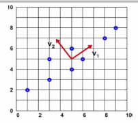 Direction of most spread of data is $$$v_{1}$$$
Perpendicular direction of $$$v_{1}$$$ is $$$v_{2}$$$
Our goal is to confirm if PCA can find direction $$$v_{1}$$$ and $$$v_{2}$$$
With given data $$$X = [x_{1}, x_{2}] = \{(1,2), (3,3), (3,5), (5,4), (5,6), (6,5), (8,7), (9,8) \}$$$,
you can find following parameters, average vector $$$\mu$$$ and covariance matrix $$$\Sigma_{X}$$$
1. $$$\mu = \begin{bmatrix} 5\\5 \end{bmatrix}$$$
1. $$$\Sigma_{X} = \frac{1}{8-1} \sum (x_{1} - \begin{bmatrix} 5\\5 \end{bmatrix})(x - \begin{bmatrix} 5\\5 \\\end{bmatrix})^{T}$$$
$$$\Sigma_{X} = \begin{bmatrix} 6.25&4.25\\4.25&3.5 \end{bmatrix}$$$
2by2 data creates 2by2 covariance matrix
@
1. You need to find eigenvalue and eigenvector
in matlab, $$$eig(\text{covariance_matrix_}\Sigma)$$$, and we get $$$\Lambda, \vec{U}$$$
Finding eigenvalue and eigenvector from 2by2 matrix is not difficult, you can try to manually find them
Definition of eigenvalue :
Eigenvalue satisfies characteristic equation $$$|\Sigma_{x}-\lambda I|=0$$$
Detail :
$$$\Sigma_{x}v=\lambda v$$$
$$$\Sigma_{x}v-\lambda v=0$$$
$$$v(\Sigma_{x}-\lambda)=0$$$
$$$v(\Sigma_{x}-\lambda I)=0$$$
To satisfy $$$v(\Sigma_{x}-\lambda I)=0$$$, v=0 or $$$(\Sigma_{x}-\lambda I)=0$$$
But v which you find shouldn't be 0 so you assume $$$(\Sigma_{x}-\lambda I)=0$$$
$$$\begin{vmatrix}\Sigma_{x}-\lambda I\end{vmatrix}=0$$$
$$$\begin{vmatrix}\begin{bmatrix} 6.25&4.25\\4.25&3.5 \end{bmatrix} - \begin{bmatrix} \lambda&0\\0&\lambda \end{bmatrix}\end{vmatrix}=0$$$
$$$\begin{vmatrix} 6.25-\lambda&4.25\\4.25&3.5-\lambda \end{vmatrix}=0$$$
You calculate determinant of 2by2 matrix by using ad-bc, then,
$$$(6.25-\lambda)(3.5-\lambda)=4.25^{2}$$$
When you solve quadratic equation in respect to $$$\lambda$$$, you can obtain 2 $$$\lambda$$$s ($$$\lambda_{1}$$$, $$$\lambda_{2}$$$)
$$$\lambda_{1}=9.34$$$
$$$\lambda_{2}=0.41$$$
You can say $$$\lambda_{1}$$$ is eigenvalue of principal component's direction
How to obtain eigenvector corresponding that direction?
You can input eigenvalues ($$$\lambda$$$ values you found from above)
into original eigenvalue/eigenvector definition formular $$$\Sigma_{x}v=\lambda v$$$
$$$\lambda_{1}=9.34$$$ results in $$$v_{11}$$$ and $$$v_{12}$$$
$$$\Sigma_{X} v = \lambda v$$$
$$$\begin{bmatrix} 6.25&4.25\\4.25&3.5 \end{bmatrix} \begin{bmatrix} v_{11}\\v_{12} \end{bmatrix} = \begin{bmatrix} \lambda_{1}v_{11}\\ \lambda_{1}v_{12} \end{bmatrix}$$$
You can obtain 2 equations
$$$6.25v_{11}+4.25v_{12}=\lambda_{1}v_{11}$$$
$$$4.25v_{11}+3.5v_{12}=\lambda_{1}v_{12}$$$
You can input $$$\lambda_{1}=9.34$$$
$$$6.25v_{11}+4.25v_{12}=9.34v_{11}$$$
$$$4.25v_{11}+3.5v_{12}=9.34v_{12}$$$
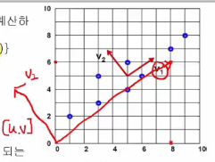
You can obtain $$$v_{11}=0.81$$$, $$$v_{12}=0.59$$$
@
You can same step with $$$\lambda_{2}$$$
$$$\Sigma_{X} v = \lambda v$$$
$$$\begin{bmatrix} 6.25&4.25\\4.25&3.5 \end{bmatrix} \begin{bmatrix} v_{21}\\v_{22} \end{bmatrix} = \begin{bmatrix} \lambda_{2}v_{21} \\ \lambda_{2}v_{22} \end{bmatrix}$$$
you can input $$$\lambda_{2}=0.41$$$ then,
$$$\begin{bmatrix} v_{21}\\ v_{22} \end{bmatrix} = \begin{bmatrix} -0.59\\0.81\end{bmatrix}$$$
$$$v_{21}=-0.59$$$
$$$v_{22}=0.81$$$
@
Let's draw vector $$$V_{1} = (v_{11},v_{12})$$$ and $$$V_{2} = (v_{21},v_{22})$$$
2018-06-06 10-54-02.png
Direction of most spread of data is $$$v_{1}$$$
Perpendicular direction of $$$v_{1}$$$ is $$$v_{2}$$$
Our goal is to confirm if PCA can find direction $$$v_{1}$$$ and $$$v_{2}$$$
With given data $$$X = [x_{1}, x_{2}] = \{(1,2), (3,3), (3,5), (5,4), (5,6), (6,5), (8,7), (9,8) \}$$$,
you can find following parameters, average vector $$$\mu$$$ and covariance matrix $$$\Sigma_{X}$$$
1. $$$\mu = \begin{bmatrix} 5\\5 \end{bmatrix}$$$
1. $$$\Sigma_{X} = \frac{1}{8-1} \sum (x_{1} - \begin{bmatrix} 5\\5 \end{bmatrix})(x - \begin{bmatrix} 5\\5 \\\end{bmatrix})^{T}$$$
$$$\Sigma_{X} = \begin{bmatrix} 6.25&4.25\\4.25&3.5 \end{bmatrix}$$$
2by2 data creates 2by2 covariance matrix
@
1. You need to find eigenvalue and eigenvector
in matlab, $$$eig(\text{covariance_matrix_}\Sigma)$$$, and we get $$$\Lambda, \vec{U}$$$
Finding eigenvalue and eigenvector from 2by2 matrix is not difficult, you can try to manually find them
Definition of eigenvalue :
Eigenvalue satisfies characteristic equation $$$|\Sigma_{x}-\lambda I|=0$$$
Detail :
$$$\Sigma_{x}v=\lambda v$$$
$$$\Sigma_{x}v-\lambda v=0$$$
$$$v(\Sigma_{x}-\lambda)=0$$$
$$$v(\Sigma_{x}-\lambda I)=0$$$
To satisfy $$$v(\Sigma_{x}-\lambda I)=0$$$, v=0 or $$$(\Sigma_{x}-\lambda I)=0$$$
But v which you find shouldn't be 0 so you assume $$$(\Sigma_{x}-\lambda I)=0$$$
$$$\begin{vmatrix}\Sigma_{x}-\lambda I\end{vmatrix}=0$$$
$$$\begin{vmatrix}\begin{bmatrix} 6.25&4.25\\4.25&3.5 \end{bmatrix} - \begin{bmatrix} \lambda&0\\0&\lambda \end{bmatrix}\end{vmatrix}=0$$$
$$$\begin{vmatrix} 6.25-\lambda&4.25\\4.25&3.5-\lambda \end{vmatrix}=0$$$
You calculate determinant of 2by2 matrix by using ad-bc, then,
$$$(6.25-\lambda)(3.5-\lambda)=4.25^{2}$$$
When you solve quadratic equation in respect to $$$\lambda$$$, you can obtain 2 $$$\lambda$$$s ($$$\lambda_{1}$$$, $$$\lambda_{2}$$$)
$$$\lambda_{1}=9.34$$$
$$$\lambda_{2}=0.41$$$
You can say $$$\lambda_{1}$$$ is eigenvalue of principal component's direction
How to obtain eigenvector corresponding that direction?
You can input eigenvalues ($$$\lambda$$$ values you found from above)
into original eigenvalue/eigenvector definition formular $$$\Sigma_{x}v=\lambda v$$$
$$$\lambda_{1}=9.34$$$ results in $$$v_{11}$$$ and $$$v_{12}$$$
$$$\Sigma_{X} v = \lambda v$$$
$$$\begin{bmatrix} 6.25&4.25\\4.25&3.5 \end{bmatrix} \begin{bmatrix} v_{11}\\v_{12} \end{bmatrix} = \begin{bmatrix} \lambda_{1}v_{11}\\ \lambda_{1}v_{12} \end{bmatrix}$$$
You can obtain 2 equations
$$$6.25v_{11}+4.25v_{12}=\lambda_{1}v_{11}$$$
$$$4.25v_{11}+3.5v_{12}=\lambda_{1}v_{12}$$$
You can input $$$\lambda_{1}=9.34$$$
$$$6.25v_{11}+4.25v_{12}=9.34v_{11}$$$
$$$4.25v_{11}+3.5v_{12}=9.34v_{12}$$$
You can obtain $$$v_{11}=0.81$$$, $$$v_{12}=0.59$$$
@
You can same step with $$$\lambda_{2}$$$
$$$\Sigma_{X} v = \lambda v$$$
$$$\begin{bmatrix} 6.25&4.25\\4.25&3.5 \end{bmatrix} \begin{bmatrix} v_{21}\\v_{22} \end{bmatrix} = \begin{bmatrix} \lambda_{2}v_{21} \\ \lambda_{2}v_{22} \end{bmatrix}$$$
you can input $$$\lambda_{2}=0.41$$$ then,
$$$\begin{bmatrix} v_{21}\\ v_{22} \end{bmatrix} = \begin{bmatrix} -0.59\\0.81\end{bmatrix}$$$
$$$v_{21}=-0.59$$$
$$$v_{22}=0.81$$$
@
Let's draw vector $$$V_{1} = (v_{11},v_{12})$$$ and $$$V_{2} = (v_{21},v_{22})$$$
2018-06-06 10-54-02.png
 @
How to reduce dimensionality
$$$W = \begin{bmatrix} | & | \\ V_{1}&V_{2} \\ | &| \end{bmatrix}$$$
$$$y=W^{T}x$$$
@
How to reduce dimensionality
$$$W = \begin{bmatrix} | & | \\ V_{1}&V_{2} \\ | &| \end{bmatrix}$$$
$$$y=W^{T}x$$$