13-02 LDA(linear discriminant analysis)
@
Projection by linear transform:
$$$y=W^{T}x$$$
W is (D,1) (D by 1)
Row vectors contained in matrix W have directions which are used when performing projection
x is (D,1)
@
2018-06-07 10-50-44.png
 One of parameters which each class has is average parameter
Red ellipse : $$$\omega_{1}$$$ class data's distribution
Blue ellipse : $$$\omega_{2}$$$ class data's distribution
Average point of each class data's distribution is generally their centroids ($$$\mu_{1}, \mu_{2}$$$)
Average of class i $$$\mu_{i}$$$ :
$$$\mu_{i} = \frac{1}{N} \sum\limits_{x\in \omega_{i}} x$$$
=========================================================
How to find average after projection?
Average of class i $$$\mu_{i}$$$ :
$$$\mu_{i} = \frac{1}{N} \sum\limits_{x\in\omega_{i}}x$$$
$$$\widetilde{\mu}_{i}$$$ : average of class i after projection
After projection means you performed linear transform $$$y=W^{T}x$$$
After that, you use function in respect to y instead of x
$$$\widetilde{\mu}_{i} = \frac{1}{N}\sum\limits_{y\in \omega_{i}}y$$$
But you can write function in respect to x again
$$$\widetilde{\mu}_{i} = \frac{1}{N}\sum\limits_{x\in \omega_{i}}W^{T}x$$$
You can write $$$W^{T}$$$ in front area
$$$\widetilde{\mu}_{i} = W^{T}\mu_{i}$$$
Meaning :
[Projection of $$$\mu_{i} = \widetilde{\mu}_{i}$$$] == [projection of $$$\omega_{1}$$$ class data -> from projected data, find its average $$$\widetilde{\mu}_{1}$$$]
2018-06-07 11-02-06.png
One of parameters which each class has is average parameter
Red ellipse : $$$\omega_{1}$$$ class data's distribution
Blue ellipse : $$$\omega_{2}$$$ class data's distribution
Average point of each class data's distribution is generally their centroids ($$$\mu_{1}, \mu_{2}$$$)
Average of class i $$$\mu_{i}$$$ :
$$$\mu_{i} = \frac{1}{N} \sum\limits_{x\in \omega_{i}} x$$$
=========================================================
How to find average after projection?
Average of class i $$$\mu_{i}$$$ :
$$$\mu_{i} = \frac{1}{N} \sum\limits_{x\in\omega_{i}}x$$$
$$$\widetilde{\mu}_{i}$$$ : average of class i after projection
After projection means you performed linear transform $$$y=W^{T}x$$$
After that, you use function in respect to y instead of x
$$$\widetilde{\mu}_{i} = \frac{1}{N}\sum\limits_{y\in \omega_{i}}y$$$
But you can write function in respect to x again
$$$\widetilde{\mu}_{i} = \frac{1}{N}\sum\limits_{x\in \omega_{i}}W^{T}x$$$
You can write $$$W^{T}$$$ in front area
$$$\widetilde{\mu}_{i} = W^{T}\mu_{i}$$$
Meaning :
[Projection of $$$\mu_{i} = \widetilde{\mu}_{i}$$$] == [projection of $$$\omega_{1}$$$ class data -> from projected data, find its average $$$\widetilde{\mu}_{1}$$$]
2018-06-07 11-02-06.png
 =========================================================
Case that you project data onto $$$x_{2}$$$ axis
2018-06-07 11-03-06.png
=========================================================
Case that you project data onto $$$x_{2}$$$ axis
2018-06-07 11-03-06.png
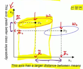 =========================================================
Distribution after projection onto each axix $$$x_{1}$$$ and $$$x_{2}$$$
2018-06-07 11-04-57.png
=========================================================
Distribution after projection onto each axix $$$x_{1}$$$ and $$$x_{2}$$$
2018-06-07 11-04-57.png
 Case you project data onto $$$x_{1}$$$ :
Wide distance between averages after projection $$$\widetilde{\mu}_{1}$$$ and $$$\widetilde{\mu}_{2}$$$
Red and blue are projected in wide range regions but they're overapped in some parts (circle on $$$x_{1}$$$)
This is good case of far distance between red class and blue class
Case you project data onto $$$x_{2}$$$ :
You get small overapped region,
which means You get more clear separation of 2 classes
This is good case of class separation
But you should achieve both of them (wide range between averages and good separation after projections)
=========================================================
You can choose "distance between average points (centroids) of each used data"
as "target function J(W)" which you should maximize :
$$$J(W) = |\widetilde{\mu}_{1} - \widetilde{\mu}_{2}|$$$
$$$J(W) = |W^{T}\mu_{1}-W^{T}\mu_{2}|$$$
$$$J(W) = |W^{T}(\mu_{1}-\mu_{2})|$$$
J(W) : target function in respect to transform matrix W
2018-06-07 11-14-47.png
Case you project data onto $$$x_{1}$$$ :
Wide distance between averages after projection $$$\widetilde{\mu}_{1}$$$ and $$$\widetilde{\mu}_{2}$$$
Red and blue are projected in wide range regions but they're overapped in some parts (circle on $$$x_{1}$$$)
This is good case of far distance between red class and blue class
Case you project data onto $$$x_{2}$$$ :
You get small overapped region,
which means You get more clear separation of 2 classes
This is good case of class separation
But you should achieve both of them (wide range between averages and good separation after projections)
=========================================================
You can choose "distance between average points (centroids) of each used data"
as "target function J(W)" which you should maximize :
$$$J(W) = |\widetilde{\mu}_{1} - \widetilde{\mu}_{2}|$$$
$$$J(W) = |W^{T}\mu_{1}-W^{T}\mu_{2}|$$$
$$$J(W) = |W^{T}(\mu_{1}-\mu_{2})|$$$
J(W) : target function in respect to transform matrix W
2018-06-07 11-14-47.png
 This target function J(W) finds most wide distance between 2 average points ($$$\widetilde{\mu}_{1}$$$ and $$$\widetilde{\mu}_{1}$$$) after projection
But this target function is insufficient in terms of finding good separation aspect,
which will be complemented by following Fisher's LDA method
=========================================================
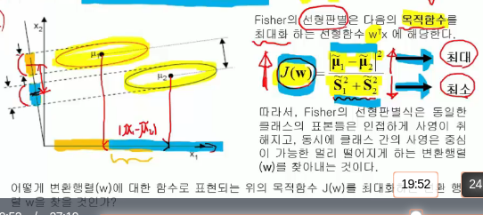
This method is suggested by Fisher
Target function J(W) which should be maximized is :
$$$J(W) = \frac{|\widetilde{\mu}_{1}-\widetilde{\mu}_{2}|^{2}}{\widetilde{S}_{1}^{2}+\widetilde{S}_{2}^{2}}$$$
$$$\widetilde{\mu}_{1}$$$ : average of class 1 data after projection
$$$\widetilde{\mu}_{2}$$$ : average of class 2 data after projection
$$$|\widetilde{\mu}_{1}-\widetilde{\mu}_{2}|^{2}$$$ : square of difference of 2 averages after projection
$$$\widetilde{S}_{1}^{2}$$$ : covariance matrix of class 1 data after projection
$$$\widetilde{S}_{2}^{2}$$$ : covariance matrix of class 2 data after projection
$$$\widetilde{S}_{1}^{2}+\widetilde{S}_{2}^{2}$$$ : indicator related to within-class scatter (variance within class)
Fisher's LDA is to find linear fucntion $$$W^{T}x$$$ which maximizes above target function J(W)
To maximize J(W),
$$$|\widetilde{\mu}_{1}-\widetilde{\mu}_{2}|^{2}$$$ should be largest
$$$\widetilde{S}_{1}^{2}+\widetilde{S}_{2}^{2}$$$ should be lowest
=========================================================
Scatter (variance) matrix of class i after projection
Since you're dealing with concept related to variance which generally is notated with squre,
you also use squre here
$$$\widetilde{S}_{i}^{2} = \sum\limits_{y\in\omega_{i}} (y-\widetilde{\mu}_{i})^{2} $$$
$$$\widetilde{S}_{i}^{2} = \sum\limits_{y\in\omega_{i}} (y-\widetilde{\mu}_{i})(y-\widetilde{\mu}_{i})^{T}$$$
=========================================================
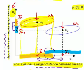
Fisher's method finds transform matrix W which projects data involved in same class onto near region,
at the same time, which makes far distances between average points after projection ($$$\tilde{\mu}_{1}, \tilde{\mu}_{2}$$$)
2018-06-07 13-08-09.png
This target function J(W) finds most wide distance between 2 average points ($$$\widetilde{\mu}_{1}$$$ and $$$\widetilde{\mu}_{1}$$$) after projection
But this target function is insufficient in terms of finding good separation aspect,
which will be complemented by following Fisher's LDA method
=========================================================
This method is suggested by Fisher
Target function J(W) which should be maximized is :
$$$J(W) = \frac{|\widetilde{\mu}_{1}-\widetilde{\mu}_{2}|^{2}}{\widetilde{S}_{1}^{2}+\widetilde{S}_{2}^{2}}$$$
$$$\widetilde{\mu}_{1}$$$ : average of class 1 data after projection
$$$\widetilde{\mu}_{2}$$$ : average of class 2 data after projection
$$$|\widetilde{\mu}_{1}-\widetilde{\mu}_{2}|^{2}$$$ : square of difference of 2 averages after projection
$$$\widetilde{S}_{1}^{2}$$$ : covariance matrix of class 1 data after projection
$$$\widetilde{S}_{2}^{2}$$$ : covariance matrix of class 2 data after projection
$$$\widetilde{S}_{1}^{2}+\widetilde{S}_{2}^{2}$$$ : indicator related to within-class scatter (variance within class)
Fisher's LDA is to find linear fucntion $$$W^{T}x$$$ which maximizes above target function J(W)
To maximize J(W),
$$$|\widetilde{\mu}_{1}-\widetilde{\mu}_{2}|^{2}$$$ should be largest
$$$\widetilde{S}_{1}^{2}+\widetilde{S}_{2}^{2}$$$ should be lowest
=========================================================
Scatter (variance) matrix of class i after projection
Since you're dealing with concept related to variance which generally is notated with squre,
you also use squre here
$$$\widetilde{S}_{i}^{2} = \sum\limits_{y\in\omega_{i}} (y-\widetilde{\mu}_{i})^{2} $$$
$$$\widetilde{S}_{i}^{2} = \sum\limits_{y\in\omega_{i}} (y-\widetilde{\mu}_{i})(y-\widetilde{\mu}_{i})^{T}$$$
=========================================================
Fisher's method finds transform matrix W which projects data involved in same class onto near region,
at the same time, which makes far distances between average points after projection ($$$\tilde{\mu}_{1}, \tilde{\mu}_{2}$$$)
2018-06-07 13-08-09.png
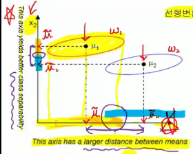
 Left axis :
short distance between average points between projected data classes
good separation
below axis ($$$x_{1}$$$) :
long distance between average points between projected data classes
bad separation (overapped)
=========================================================
How to find transform matrix W which maximizes target function J(W)?
That method is already found by mathematicians
Target function J(W) you've seen is this :
$$$J(W) = \frac{|\widetilde{\mu}_{1}-\widetilde{\mu}_{2}|^{2}}{\widetilde{S}_{1}^{2}+\widetilde{S}_{2}^{2}}$$$
To find optimal transform matrix W, you need to express target function J(W) in respect to W
Assumption :
In multi-dimension feature space, scatter matrix S is identical form to covariance matrix only without scale factor $$$\frac{1}{N-1}$$$
Scatter matrix of class i $$$S_{i} = \sum\limits_{x\in\omega_{i}} (x-\mu_{i}) (x-\mu_{i})^{T}$$$
2018-06-07 13-19-48.png
Left axis :
short distance between average points between projected data classes
good separation
below axis ($$$x_{1}$$$) :
long distance between average points between projected data classes
bad separation (overapped)
=========================================================
How to find transform matrix W which maximizes target function J(W)?
That method is already found by mathematicians
Target function J(W) you've seen is this :
$$$J(W) = \frac{|\widetilde{\mu}_{1}-\widetilde{\mu}_{2}|^{2}}{\widetilde{S}_{1}^{2}+\widetilde{S}_{2}^{2}}$$$
To find optimal transform matrix W, you need to express target function J(W) in respect to W
Assumption :
In multi-dimension feature space, scatter matrix S is identical form to covariance matrix only without scale factor $$$\frac{1}{N-1}$$$
Scatter matrix of class i $$$S_{i} = \sum\limits_{x\in\omega_{i}} (x-\mu_{i}) (x-\mu_{i})^{T}$$$
2018-06-07 13-19-48.png
 Note
Covariance matrix $$$\Sigma= \frac{1}{N-1} \sum\limits_{x\in\omega_{i}} (x-\mu_{i}) (x-\mu_{i})^{T}$$$
Scatter matrix within class S_{with-in-class} :
$$$S_{with-in-class}^{2} = S_{1}^{2} + S_{2}^{2}$$$
=========================================================
After projection, scatter matrix within class \widetilde{S}_{with-in-class} has following relation
$$$\widetilde{S}_{1}^{2} + \widetilde{S}_{2}^{2} = W^{T}S_{within-class}W = \widetilde{S}_{within-class}$$$
$$$S_{within-class}$$$ : scatter matrix (covariance matrix) within class before projection
W : tranform matrix
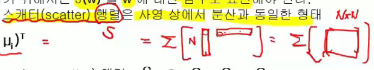
Induce step :
$$$\widetilde{S}_{i}^{2} = \sum\limits_{y\in\omega_{i}} (y-\widetilde{\mu}) (y-\widetilde{\mu})^{T}$$$
$$$\widetilde{S}_{i}^{2} = \sum\limits_{x\in\omega_{i}} (W^{T}x-W^{T}\mu_{i}) (W^{T}x-W^{T}\mu_{i})^{T}$$$
$$$\widetilde{S}_{i}^{2} = \sum\limits_{x\in\omega_{i}} W^{T} (x-\mu_{i}) (x-\mu_{i})^{T} W$$$
$$$\widetilde{S}_{i}^{2} = W^{T}S_{i}^{2}W$$$
Note
Covariance matrix $$$\Sigma= \frac{1}{N-1} \sum\limits_{x\in\omega_{i}} (x-\mu_{i}) (x-\mu_{i})^{T}$$$
Scatter matrix within class S_{with-in-class} :
$$$S_{with-in-class}^{2} = S_{1}^{2} + S_{2}^{2}$$$
=========================================================
After projection, scatter matrix within class \widetilde{S}_{with-in-class} has following relation
$$$\widetilde{S}_{1}^{2} + \widetilde{S}_{2}^{2} = W^{T}S_{within-class}W = \widetilde{S}_{within-class}$$$
$$$S_{within-class}$$$ : scatter matrix (covariance matrix) within class before projection
W : tranform matrix
Induce step :
$$$\widetilde{S}_{i}^{2} = \sum\limits_{y\in\omega_{i}} (y-\widetilde{\mu}) (y-\widetilde{\mu})^{T}$$$
$$$\widetilde{S}_{i}^{2} = \sum\limits_{x\in\omega_{i}} (W^{T}x-W^{T}\mu_{i}) (W^{T}x-W^{T}\mu_{i})^{T}$$$
$$$\widetilde{S}_{i}^{2} = \sum\limits_{x\in\omega_{i}} W^{T} (x-\mu_{i}) (x-\mu_{i})^{T} W$$$
$$$\widetilde{S}_{i}^{2} = W^{T}S_{i}^{2}W$$$