% https://www.youtube.com/watch?v=dIKri3LjWpY&index=23&t=0s&list=PLbhbGI_ppZIRPeAjprW9u9A46IJlGFdLn % 002_Dirhichlet_Process_002.py % === % 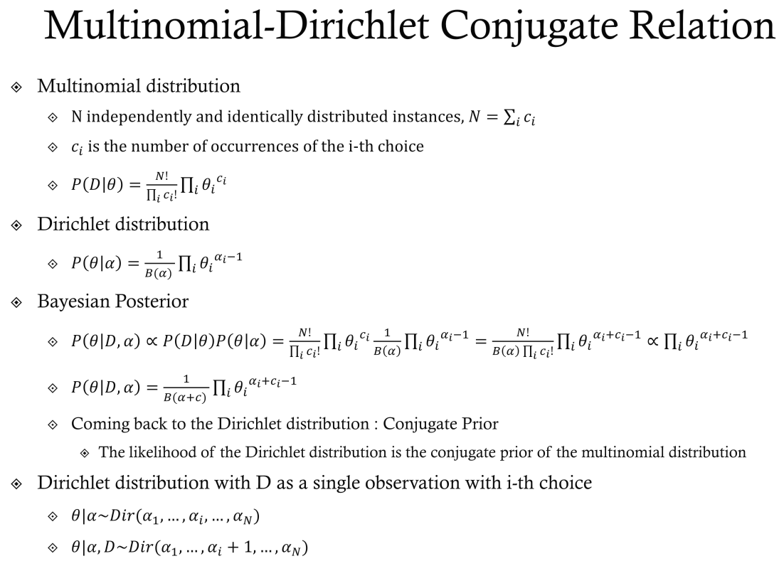Relation (conjugate relation) between multinomial distribution and Dirichlet distribution Let's write multinomial distribution $$$P(D|\theta) = \dfrac{N!}{\prod_i c_i!} \prod_i \theta_i^{c_i}$$$ $$$\dfrac{N!}{\prod_i c_i!}$$$: normalize constant which is applied when you have multiple trials $$$\theta_i^{c_i}$$$: more important part $$$\theta_i$$$: probability of occurring $$$\theta$$$ from i-th selection $$$c_i$$$: when $$$\theta$$$ is multiple selected $$$\prod_i$$$: since you have i number of options % === Let's write Dirichlet distribution $$$P(\theta|\alpha) = \dfrac{1}{B(\alpha)} \prod_i \theta_i^{\alpha_i-1}$$$ $$$B(\alpha)$$$: simplified notation, actually more complicated form Important point is that parameter $$$\alpha$$$ from $$$P(\theta|\alpha)$$$ is located in $$$\theta_i^{\alpha_i-1}$$$ Common point is that $$$c_i$$$ and $$$\alpha_i-1$$$ are located in exponent part from Multinomial and Dirichlet distributions But note that $$$\theta$$$ is given in Multinomial distribution and $$$\theta$$$ is being created in Dirichlet distribution You can see good combination from above two distribution If this $$$P(D|\theta)P(\theta|\alpha)$$$ happens exponent parts can be summed Or by using $$$\theta$$$ as medium you can explain $$$P(D|\alpha)$$$ (when given prior $$$\alpha$$$, explain data D) % === $$$P(D|\theta)$$$ is likelihood form $$$P(\theta|\alpha)$$$ is prior form Posterior form $$$\propto P(D|\theta)P(\theta|\alpha)$$$ Posterior form is what you always want to find especially when you update parameters % === You can find posterior wrt parameter $$$\theta$$$ $$$P(\theta|D,\alpha)$$$ like this $$$P(\theta|D,\alpha) \propto P(D|\theta)P(\theta|\alpha)$$$ So, you can write $$$P(\theta|D,\alpha) \propto \dfrac{N!}{\prod_i c_i!} \prod_i \theta_i^{c_i} \dfrac{1}{B(\alpha)} \prod_i \theta_i^{\alpha_i-1}$$$ You can sum exponent parts $$$P(\theta|D,\alpha) \propto \dfrac{N!}{B(\alpha)\prod_i c_i!} \prod_i \theta_i^{\alpha_i+c_i-1} $$$ And you can write proportion because $$$\dfrac{N!}{B(\alpha)\prod_i c_i!}$$$ is normalize constant $$$\dfrac{N!}{B(\alpha)\prod_i c_i!} \prod_i \theta_i^{\alpha_i+c_i-1} \propto \prod_i\theta_i^{\alpha_i+c_i-1}$$$ % === $$$\prod_i\theta_i^{\alpha_i+c_i-1}$$$ is same form with Dirichlet definition $$$P(\theta|\alpha) = \dfrac{1}{B(\alpha)} \prod_i \theta_i^{\alpha_i-1}$$$ You need to edit $$$\alpha$$$ and $$$\alpha_i-1$$$ from $$$\dfrac{1}{B(\alpha)} \prod_i \theta_i^{\alpha_i-1}$$$ to sync Updated form $$$P(\theta|D,\alpha) = \dfrac{1}{B(\alpha+c)} \prod_i \theta_i^{\alpha_i+c_i-1}$$$ In conclusion, prior is Dirichlet and likelihood is multinomial and posterior is Dirichlet So, you will call "coming back to Dirichlet distribution" as "conjugate prior" So, to keep conjugate prior relation, you use Dirichlet distribution in LDA % === Data D is count of selection $$$N=\sum_i c_i$$$ $$$c_i$$$ is number of occurrences of i-th choice Data D is composed of c Data is applied to prior $$$\alpha$$$ from $$$\prod_{i} \theta_i^{\alpha_i+c_i-1}$$$ This process is called Bayesian or belief update % === If Dirichlet distribution with data D as single observation with i-th choice Count N is 1, remains are 0 Parameter $$$\theta$$$ ($$$\theta|\alpha $$$) is created by being sampled via Dirichlet distribution $$$Dir(\alpha_1,...,\alpha_i,...,\alpha_N)$$$ Parameter $$$\theta$$$ ($$$\theta|\alpha,D $$$ with data D) is created by being sampled via Dirichlet distribution $$$Dir(\alpha_1,...,\alpha_i+1,...,\alpha_N)$$$ +1 means observed choice (data D) $$$\theta|\alpha$$$ will be prior $$$P(\theta|\alpha)$$$ $$$\theta|\alpha,D$$$ will be posterior And posterior is still Dirichlet distribution and posterior can be used as prior to update