This is note from the following video lecture https://www.youtube.com/watch?v=nMAtFhamoRY ================================================================================ True Positive, True Negative, False Positive, False Negative True, False: predicton of your model is correct or incorrect Positive, Negative: 1 and 0 in classes ================================================================================
1000 pics in total Model predicted it's non-tumor Model predicted it's tumor
On non-tumor pics 988 (True Negative) 2 (False Positive)
On tumor pics 1 (False Negative) 9 (True Positive)
True Negative: The model correctly said 988 non-tumor images would be non-tumor images False Positive: The model incorrectly said 2 non-tumor images would be tumor images False Negative: The model incorrectly said 1 tumor image would be non-tumor image True Positive: The model correctly said 9 tumor images would be tumor images Above table corresponds to following confusion matrix (binary confusion matrix specifically because you have binary class in this example) [[988,2], [1,9]] ================================================================================ $$$\text{Accuracy}$$$ $$$=\frac{\text{TP}+\text{TN}}{\text{All cases}} $$$ $$$=\frac{9+988}{1000}$$$ $$$=0.99$$$ $$$\text{Precison}$$$ $$$=\frac{\text{TP}}{\text{TP}+\text{FP}} $$$ $$$=\frac{9}{9+2}$$$ $$$=0.81$$$ $$$\text{Recall}$$$ $$$=\frac{\text{TP}}{\text{TP}+\text{FN}} $$$ $$$=\frac{9}{9+1}$$$ $$$=0.9$$$ ================================================================================ In addition to accuracy, precision, recall, you will see ROC curve. ROC curve is much used for binary classification and medical appications. You can calculate confusion matrix by using scikit-learn Or you can manually calculate it ================================================================================ How can you interpret ROC curve? Red curve line has better performance. Area under curve line is called AUC (Area Under the Curve). ================================================================================ Why do you need to use ROC curve? Precision and recall are used to complement the weak point of accuracy. ROC is also used to inspect analyzed result and dataset. ================================================================================ Probability distribution N means distribution of non-tumor images Probability distribution P means distribution of tumor images You can see clearly separated areas like far-left and far-right but note that there are kind of unclear or overlapped areas around the center area. Even if you have those unclear and overlapped areas, you should have the best separating line like green vertical line It means you can't avoid the errors in your separating line or in your decision. ================================================================================ This graph is more easily separable. Even if green vertical line moves in this graph, you won't have many miss classifications because graph is already quite clear separable. (decision boundary is less sensitive, you can more trust that you can separate N and P , you have good feature to separate N and P) This situatino draws red-line-like graph in ROC curve. ================================================================================ If graph is not easily separable, almost-straight-diagonal-line is plotted on the ROC curve, which is bad curve. ================================================================================ So, it means you can use ROC curve to select good features ================================================================================ For example, suppose you want to predict fast runners. To train the mode, suppose you select "weight" and "height" as features. But there are many vague cases where some tall people run fast, some tall people run slow, some overweight people run fast, some lightweight people run fast, etc. This situation draw distribution like and draw almost-straight-diagonal-line on ROC curve ================================================================================ When you use good feature like record in previous test, you can separate people into fast runner and slow runner And that situation will draw following distribution and red-line-like good curve on ROC curve ================================================================================ True Positive rate (= Recall, sensitivity) $$$\text{TPR=R}$$$ $$$=\frac{\text{TP}}{\text{TP}+\text{FN}}$$$ ================================================================================ True Negative rate (= Specificity) $$$\text{TNR}$$$ $$$=\frac{\text{TN}}{\text{TN}+\text{FP}}$$$ ================================================================================ Summary 1. Accuracy is not all Especiialy, when class is inbalanced, you should see precision and recall For example, first medical inspection should use recall cause it should detect every tumor patient. Precision should be used for the case where your judgement shouldn't have mistake such as conviction. 2. Use ROC curve to confirm that you're using good features, your decision is reliable and stable judgement by checking your AUC has large area ================================================================================ Calcuate metrics by using Scikit-learn libray and by using manual calculation
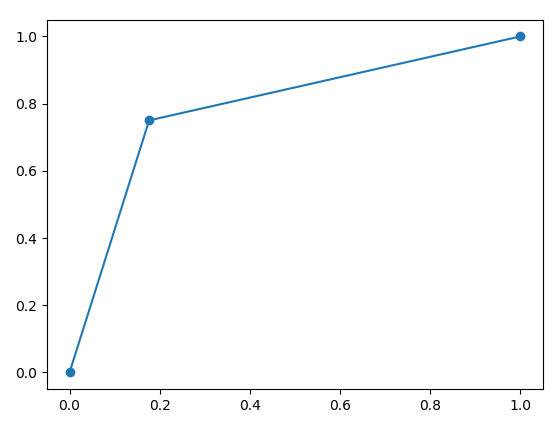
# ================================================================================
# @ 1. Calculate confusion matrix
from sklearn.metrics import confusion_matrix

y_true=[0, 0, 0, 1, 0, 1, 0, 1, 0, 0, 0, 0, 0, 0, 0, 0, 1, 0, 0, 0, 0, 0, 1, 0, 1, 
        0, 1, 0, 1, 1, 1, 1, 0, 0, 1, 0, 0, 0, 0, 1, 0, 1, 0, 1, 1, 1, 0, 0, 1, 1, 
        0, 0, 0, 1, 0, 0, 1, 0, 0, 0, 0, 0, 0, 0, 0, 0, 1, 0, 0, 0, 0, 1, 0, 0, 1, 
        0, 0, 0, 1, 0, 1, 0, 1, 1, 0, 1, 0, 0, 1, 1, 0, 0, 0, 1, 0, 0, 0, 0, 0, 0]
y_pred=[0, 0, 0, 1, 0, 1, 1, 1, 0, 0, 0, 0, 1, 1, 0, 0, 1, 0, 0, 0, 0, 0, 1, 0, 0, 
        1, 0, 0, 1, 0, 1, 0, 0, 0, 1, 1, 0, 0, 0, 1, 0, 1, 0, 1, 1, 1, 0, 0, 1, 0, 
        0, 0, 0, 1, 1, 0, 1, 1, 0, 0, 0, 1, 0, 0, 0, 0, 1, 0, 0, 1, 0, 0, 0, 0, 1, 
        0, 0, 1, 1, 0, 1, 0, 0, 1, 0, 1, 0, 0, 1, 0, 0, 0, 0, 1, 0, 1, 0, 1, 0, 0]

c_mat=confusion_matrix(y_true,y_pred,labels=[1,0])
print(c_mat)
# [[24  8]
#  [12 56]]

# ================================================================================
# @ 2. Calculate various metrics using classification_report()

from sklearn.metrics import classification_report
classification_report_result=classification_report(
   y_true,y_pred,target_names=['class Non tumor (neg)','class Tumor (pos)'])
print("classification_report_result",classification_report_result)
#                        precision    recall  f1-score   support

# class Non tumor (neg)       0.88      0.82      0.85        68
#     class Tumor (pos)       0.67      0.75      0.71        32

#             micro avg       0.80      0.80      0.80       100
#             macro avg       0.77      0.79      0.78       100
#          weighted avg       0.81      0.80      0.80       100

# ================================================================================
# @ 3. Calculate metrics one by one

from sklearn.metrics import accuracy_score,precision_score,
                            recall_score,fbeta_score,f1_score

print("accuracy_score",accuracy_score(y_true,y_pred).astype("float16"))
# 0.8

print("precision_score",precision_score(y_true,y_pred).astype("float16"))
# 0.6665

print("recall_score",recall_score(y_true,y_pred).astype("float16"))
# 0.75

# print("fbeta_score",fbeta_score(y_true, y_pred, beta))

print("f1_score",fbeta_score(y_true,y_pred,beta=1).astype("float16"))
# 0.706

# ================================================================================
# @ 4. Calculate ROC curve

from sklearn.metrics import roc_curve
import matplotlib.pyplot as plt

fpr,tpr,thresholds=roc_curve(y_true,y_pred)
plt.plot(fpr,tpr,'o-')
plt.show()
It turns out AUC has large area ================================================================================
# @ Calculate metrics manually

import numpy as np

y_true_np=np.array(y_true)
y_pred_np=np.array(y_pred)

# ================================================================================
mask_for_diff=y_pred_np!=y_true_np
y_true_diff_against_y_pred=y_true_np[mask_for_diff]
y_pred_diff_against_y_true=y_pred_np[mask_for_diff]
# print(y_true_diff_against_y_pred)
# [0 0 0 1 0 1 1 1 0 1 0 0 0 0 1 0 1 1 0 0]
# print(y_pred_diff_against_y_true)
# [1 1 1 0 1 0 0 0 1 0 1 1 1 1 0 1 0 0 1 1]

num_of_what_pred_said_1_incorrectly_in_diff_cases=np.sum((y_pred_diff_against_y_true==1).astype("uint8"))
num_of_what_pred_said_0_incorrectly_in_diff_cases=np.sum((y_pred_diff_against_y_true==0).astype("uint8"))
# print(num_of_what_pred_said_1_incorrectly_in_diff_cases)
# 12
# print(num_of_what_pred_said_0_incorrectly_in_diff_cases)
# 8

# ================================================================================
mask_for_same=y_pred_np==y_true_np
y_pred_same_against_y_true=y_pred_np[mask_for_same]
y_true_same_against_y_pred=y_true_np[mask_for_same]
# print(y_pred_same_against_y_true)
# [0 0 0 1 0 1 1 0 0 0 0 0 0 1 0 0 0 0 0 1 0 0 1 1 0 0 1 0 0 0 1 0 1 0 1 1 1
#  0 0 1 0 0 0 1 0 1 0 0 0 0 0 0 0 1 0 0 0 0 0 1 0 0 1 0 1 0 1 0 1 0 0 1 0 0
#  0 1 0 0 0 0]
# print(y_true_same_against_y_pred)
# [0 0 0 1 0 1 1 0 0 0 0 0 0 1 0 0 0 0 0 1 0 0 1 1 0 0 1 0 0 0 1 0 1 0 1 1 1
#  0 0 1 0 0 0 1 0 1 0 0 0 0 0 0 0 1 0 0 0 0 0 1 0 0 1 0 1 0 1 0 1 0 0 1 0 0
#  0 1 0 0 0 0]

num_of_what_pred_said_1_correctly_in_same_cases=np.sum((y_pred_same_against_y_true==1).astype("uint8"))
num_of_what_pred_said_0_correctly_in_same_cases=np.sum((y_pred_same_against_y_true==0).astype("uint8"))
# print(num_of_what_pred_said_1_correctly_in_same_cases)
# 24
# print(num_of_what_pred_said_0_correctly_in_same_cases)
# 56

# ================================================================================
# @ 5. Calculate binary confusion matrix manually

True_Positive=num_of_what_pred_said_1_correctly_in_same_cases
False_Positive=num_of_what_pred_said_0_incorrectly_in_diff_cases
False_Negative=num_of_what_pred_said_1_incorrectly_in_diff_cases
True_Negative=num_of_what_pred_said_0_correctly_in_same_cases

confusion_mat=[
  [True_Positive,False_Positive],
  [False_Negative,True_Negative]]
print(confusion_mat)
# [[24, 8],
#  [12, 56]]

# ================================================================================
# @ 6. Calculate accuracy, precision, recall manually

# (1) Accuracy
accracy=(True_Positive+True_Negative)/(True_Positive+False_Positive+False_Negative+True_Negative)
print(accracy.astype("float16"))
# 0.8

# (2) Precision
precision=True_Positive/(True_Positive+False_Positive)
print(precision.astype("float16"))
# 0.75

# (2) Recall
recall=True_Positive/(True_Positive+False_Negative)
print(recall.astype("float16"))
# 0.6665