004-003. neural network basic - word2vec
import tensorflow as tf
import matplotlib
import matplotlib.pyplot as plt
import numpy as np
# This configuration lets korean language show in matplotlib
font_name=matplotlib.font_manager\
.FontProperties(fname="/media/young/5e7be152-8ed5-483d-a8e8-b3fecfa221dc/font/NanumFont/NanumGothic.ttf")\
.get_name()
matplotlib.rc('font',family=font_name)
# You will vectorize following sentences
sentences=["나 고양이 좋다",
"나 강아지 좋다",
"나 동물 좋다",
"강아지 고양이 동물",
"여자친구 고양이 강아지 좋다",
"고양이 생선 우유 좋다",
"강아지 생선 싫다 우유 좋다",
"강아지 고양이 눈 좋다",
"나 여자친구 좋다",
"여자친구 나 싫다",
"여자친구 나 영화 책 음악 좋다",
"나 게임 만화 애니 좋다",
"고양이 강아지 싫다",
"강아지 고양이 좋다"]
# 문장을 전부 합친 후 공백으로 단어들을 나누고 고유한 단어들로 리스트를 만듭니다.
# You merge all elements in "sentences" with delimiter " ",
# and then, split merged one
word_sequence=" ".join(sentences).split()
# < '나 고양이 좋다 나 강아지 좋다 나 동물 좋다 강아지 고양이 동물 여자친구 고양이 강아지 좋다 고양이 생선 우유 좋다 강아지 생선 싫다 우유 좋다 강아지 고양이 눈 좋다 나 여자친구 좋다 여자친구 나 싫다 여자친구 나 영화 책 음악 좋다 나 게임 만화 애니 좋다 고양이 강아지 싫다 강아지 고양이 좋다'
# < ['나',
# < '고양이',
# < '좋다',
# < '나',
# < '강아지',
# < '좋다',
# < '나',
# < '동물',
# < '좋다',
# < '강아지',
# < '고양이',
# < '동물',
# < '여자친구',
# < '고양이',
# < '강아지',
# < '좋다',
# < '고양이',
# < '생선',
# < '우유',
# < '좋다',
# < '강아지',
# < '생선',
# < '싫다',
# < '우유',
# < '좋다',
# < '강아지',
# < '고양이',
# < '눈',
# < '좋다',
# < '나',
# < '여자친구',
# < '좋다',
# < '여자친구',
# < '나',
# < '싫다',
# < '여자친구',
# < '나',
# < '영화',
# < '책',
# < '음악',
# < '좋다',
# < '나',
# < '게임',
# < '만화',
# < '애니',
# < '좋다',
# < '고양이',
# < '강아지',
# < '싫다',
# < '강아지',
# < '고양이',
# < '좋다']
word_list=" ".join(sentences).split()
word_list=list(set(word_list))
# Since it's easier to analyze text with number than character,
# you will create correlation array,
# and index array which allows you to reference word in word list,
# to use index of character in list
# < ['나',
# < '고양이',
# < '좋다',
# < '나',
# < '강아지',
# < '좋다',
# < '나',
# < '동물',
# < '좋다',
# < '강아지',
# < '고양이',
# < '동물',
# < '여자친구',
# < '고양이',
# < '강아지',
# < '좋다',
# < '고양이',
# < '생선',
# < '우유',
# < '좋다',
# < '강아지',
# < '생선',
# < '싫다',
# < '우유',
# < '좋다',
# < '강아지',
# < '고양이',
# < '눈',
# < '좋다',
# < '나',
# < '여자친구',
# < '좋다',
# < '여자친구',
# < '나',
# < '싫다',
# < '여자친구',
# < '나',
# < '영화',
# < '책',
# < '음악',
# < '좋다',
# < '나',
# < '게임',
# < '만화',
# < '애니',
# < '좋다',
# < '고양이',
# < '강아지',
# < '싫다',
# < '강아지',
# < '고양이',
# < '좋다']
word_dict={w: i for i,w in enumerate(word_list)}
# < {'강아지': 9,
# < '게임': 8,
# < '고양이': 2,
# < '나': 0,
# < '눈': 6,
# < '동물': 15,
# < '만화': 3,
# < '생선': 10,
# < '싫다': 13,
# < '애니': 4,
# < '여자친구': 1,
# < '영화': 14,
# < '우유': 7,
# < '음악': 5,
# < '좋다': 11,
# < '책': 12}
# You will create skip-gram model whose window size is 1
# For example, 나 게임 만화 애니 좋다,
# [나,만화] is feature
# 게임 is label
# -> ([나,만화],게임),([게임,애니],만화),([만화,좋다],애니)
# -> (게임,나),(게임,만화),(만화,게임),(만화,애니),(애니,만화),(애니,좋다)
skip_grams=[]
# len(word_sequence) is 52
for i in range(1,len(word_sequence) - 1):
# (context,target):([target index-1,target index+1],target)
# After you create skip-gram, you save index of word
# word_sequence[1] is '고양이'
# target=2
target=word_dict[word_sequence[i]]
# word_dict[word_sequence[i-1]]=1
# word_dict[word_sequence[2]]=11
# context=[1,11]
context=[word_dict[word_sequence[i-1]],word_dict[word_sequence[i+1]]]
for w in context:
# skip_grams=[[2,[1,11]], ...]
skip_grams.append([target,w])
# This method generates batch data of input and ouput,
# by randomly extracting data from skip-gram data
def random_batch(data,size):
random_inputs=[]
random_labels=[]
random_index=np.random.choice(range(len(data)),size,replace=False)
for i in random_index:
# This extracts target
random_inputs.append(data[i][0])
# This extracts context
random_labels.append([data[i][1]])
return random_inputs,random_labels
# @
# You will configure options
training_epoch=10000
learning_rate=0.1
batch_size=20
# Word vector is composed of embedding
# embedding_size is size of its dimension
# You will use 2 dimension embedding for word vector,
# to easily express embeddings onto xy plane
embedding_size=2
# This is size of sampling which is used in nce_loss(),
# when you train word2vec model
# This value should be smaller than batch_size
num_sampled=15
# voc_size means entire number of word
voc_size=len(word_list)
# @
# You will build neural network model
# This is placeholder for inputs
inputs=tf.placeholder(tf.int32,shape=[batch_size])
# When you use tf.nn.nce_loss(), you should configure output label as [batch_size,1]
labels=tf.placeholder(tf.int32,shape=[batch_size,1])
# This variable will store embedding vectors which are result of word2vec model
# This is composed of voc_size*embedding_size matrix
# They're voc_size and embedding_size
embeddings=tf.Variable(tf.random_uniform([voc_size,embedding_size],-1.0,1.0))
# embeddings inputs selected_embed
# [[1,2,3] -> [2,3] -> [[2,3,4]
# [2,3,4] [3,4,5]]
# [3,4,5]
# [4,5,6]]
selected_embed=tf.nn.embedding_lookup(embeddings,inputs)
# You define parameters which will be used in nce_loss()
nce_weights=tf.Variable(tf.random_uniform([voc_size,embedding_size],-1.0,1.0))
nce_biases=tf.Variable(tf.zeros([voc_size]))
# It's complex to directly implement nce_loss()
# You just can use tf.nn.nce_loss() provided by tf
# You create loss function in nce_loss function
loss=tf.reduce_mean(
tf.nn.nce_loss(nce_weights,nce_biases,labels,selected_embed,num_sampled,voc_size))
# You create optimizer
train_op=tf.train.AdamOptimizer(learning_rate).minimize(loss)
# @
# You will train your neural network model
# You open session
with tf.Session() as sess:
# You initialize variables
init=tf.global_variables_initializer()
sess.run(init)
# You let model to train
for step in range(1,training_epoch+1):
batch_inputs,batch_labels=random_batch(skip_grams,batch_size)
# train_op is optimizer
# loss is nce_loss function
# loss_val is loss value
_,loss_val=sess.run([train_op,loss],
feed_dict={inputs: batch_inputs,
labels: batch_labels})
# You display loss value every 10 step
if step % 10 == 0:
print("loss at step ",step,": ",loss_val)
# < loss at step 10 : 4.640656
# < loss at step 20 : 3.7076352
# < loss at step 30 : 3.4454236
# < loss at step 40 : 3.92434
# < loss at step 50 : 3.4112315
# < loss at step 60 : 3.3955512
# < loss at step 70 : 3.7334003
# < loss at step 80 : 3.1573186
# < loss at step 90 : 3.304488
# < loss at step 100 : 3.2934136
# < loss at step 110 : 3.2376626
# < loss at step 120 : 3.4271011
# < loss at step 130 : 3.2045867
# < loss at step 140 : 3.0137382
# < loss at step 150 : 3.2337089
# < loss at step 160 : 3.1725814
# < loss at step 170 : 3.4625728
# < loss at step 180 : 3.30521
# < loss at step 190 : 3.3242996
# < loss at step 200 : 3.1565833
# < loss at step 210 : 3.363378
# < loss at step 220 : 3.2673995
# < loss at step 230 : 3.2842145
# < loss at step 240 : 3.1075568
# < loss at step 250 : 3.4219444
# < loss at step 260 : 3.293485
# < loss at step 270 : 3.12632
# < loss at step 280 : 3.1017227
# < loss at step 290 : 3.2007794
# < loss at step 300 : 3.1695514
# You save value of embeddings,
# to visualize it by matplotlib
# You simply can use eval() instead of sess.run in with statement
trained_embeddings=embeddings.eval()
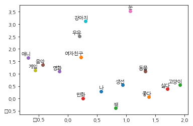
# @
# You will see word2vec where words are embedded into
# Result shows how much specific word is correlated with other words
for i,label in enumerate(word_list):
x,y=trained_embeddings[i]
plt.scatter(x,y)
plt.annotate(label,xy=(x,y),xytext=(5,2),
textcoords='offset points',ha='right',va='bottom')
plt.show()
# img 2ea47a3c-a824-4e74-8e93-828715782233