https://www.youtube.com/watch?v=NMesGSXr8H4
================================================================================
Many domains to which RL is applied are MDP
RL is about how to find optimal decision making in MDP
================================================================================
Outline
(1) Markov processes
(2) Markov reward processes: Markov processes + reward
(3) Markov decision processes: Markov processes + reward + action
(4) Extensions to MDPs
================================================================================
* Markov decision processes (MDP) formally describe an environment for RL
* MDP means the environment is fully observable
* For example, current state completely characterizes (or express) the process
* Almost all RL problems can be formalised as MDPs problem
(1) Optimal control primarily deals with continuous MDPs
(2) Partially observable problems can be converted into MDPs
(3) Bandits are MDPs with one state
================================================================================
Markov property (Markov state)
* The future is independent of the past given the preseent
* $$$\mathbb{P}[S_{t+11}|S_t] = \mathbb{P}[S_{t+1}|S_1,\cdots,S_t]$$$
$$$S_t$$$: state
* The state $$$S_t$$$ captures "all relevant information" from the history
* Once the state is known, the history may be thrown awat
* i.e., the state is a sufficient static of the future
================================================================================
State transition matrix
* Environment has state transition matrix
* State transition matrix is used to explain environment
* State transition matrix is used for MP, MRP, MDP
* Markov processes don't have "action"
* Agent in markov processes goes next state based on "fixed probability"
* At state $$$s$$$ at time $$$t$$$,
there are many candidate states $$$s^{'}$$$ at time $$$t+1$$$
* State transition matrix contains probabilities of transition from $$$s$$$ to $$$s^{'}$$$
* State transition probability from $$$s$$$ to $$$s^{'}$$$
For a "Markov state s" and "successor state $$$s^{'}$$$",
the "state transition probability" is defined by
$$$\mathcal{P}_{ss^{'}} = \mathbb{P}[S_{t+1}=s^{'}|S_t=s]$$$
* State transition matrix:
state transition matrix \mathcal{P} defines "transition probabilities"
from all state s to all success state $$$s^{'}$$$
$$$\mathcal{P} = \text{from} \;\;
\begin{bmatrix}
\mathcal{P}_{11}&&\cdots&&\mathcal{P}_{1n}\\
\vdots&&&&\vdots\\
\mathcal{P}_{n1}&&\cdots&&\mathcal{P}_{nn}\\
\end{bmatrix}$$$
- $$$\mathcal{P}_{11}$$$: probability of transition from state 1st to state 1st
- $$$\mathcal{P}_{nn}$$$: probability of transition from state nth to state nth
- n number of states
- States are discrete
================================================================================
Markov process
* Markov process can be defined by "state" and "transition probability"
* Definition of markov process (or markov chain): tuple of $$$\langle \mathcal{S},\mathcal{P} \rangle$$$
- $$$\mathcal{S}$$$: (finite) set of all states, $$$\mathcal{S}=\{S_1,S_2,\cdots\}$$$
- $$$\mathcal{P}$$$: state transition probability matrix,
- $$$\mathcal{P}_{ss^{'}}=\mathbb{P}[S_{t+1}=s^{'}|S_t=s]$$$
* Markov process is a memoryless random process
(1) Memoryless: Regardless of paths agent walked through,
one agent arrives state s, future of agent is defined by transition probability
(2) Random process: sampling is possible
Suppose agent stays at state s.
Agents moves from state to state.
Historical record of states is created
But even if agent starts with same initial state, historical record of states can be different
================================================================================
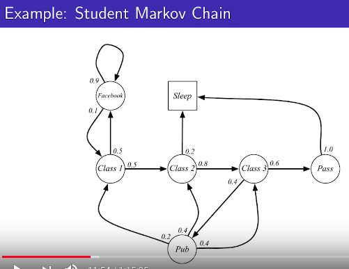 * Example of markov process
* Number of states: 7
* State transition probability: arrow and number
* Sleep: terminal state
================================================================================
* Example of markov process
* Number of states: 7
* State transition probability: arrow and number
* Sleep: terminal state
================================================================================
 * Do sampling on episodes
* Episode: starting state to termnal state
* You sample 1st episode: C1 C2 C3 Pass Sleep
* You sample 2nd episode: C1 FB FB C1 C2 Sleep
================================================================================
* Do sampling on episodes
* Episode: starting state to termnal state
* You sample 1st episode: C1 C2 C3 Pass Sleep
* You sample 2nd episode: C1 FB FB C1 C2 Sleep
================================================================================
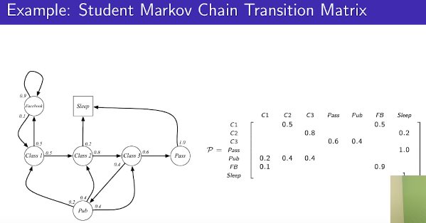 Markov chain transition matrix
* Markov processes are defined by set of states and transition matrix
================================================================================
Markov processes is about dynamics of environment in RL
Dynamic: environment is working in what mechanism
================================================================================
* Markov reward process (MRP) is markov process (markov chain) + reward (value)
* MRP is defined by 4 length tuple, $$$\langle \mathcal{S},\mathcal{P},\mathcal{R},\gamma \rangle$$$
* $$$\mathcal{S}$$$: set of states
* $$$\mathcal{P}$$$: state transition probability matrix
$$$\mathcal{P}_{ss^{'}} = \mathbb{P}[S_{t+1}=s^{'}|S_t=s]$$$
* $$$\mathcal{R}$$$: reward function, $$$\mathcal{R}_s = \mathbb{P}[R_{t+1}|S_t=s]$$$
reward_value=reward_function_for_each_state(state)
* $$$\gamma$$$: discount factor, $$$\gamma \in [0,1]$$$
================================================================================
Markov chain transition matrix
* Markov processes are defined by set of states and transition matrix
================================================================================
Markov processes is about dynamics of environment in RL
Dynamic: environment is working in what mechanism
================================================================================
* Markov reward process (MRP) is markov process (markov chain) + reward (value)
* MRP is defined by 4 length tuple, $$$\langle \mathcal{S},\mathcal{P},\mathcal{R},\gamma \rangle$$$
* $$$\mathcal{S}$$$: set of states
* $$$\mathcal{P}$$$: state transition probability matrix
$$$\mathcal{P}_{ss^{'}} = \mathbb{P}[S_{t+1}=s^{'}|S_t=s]$$$
* $$$\mathcal{R}$$$: reward function, $$$\mathcal{R}_s = \mathbb{P}[R_{t+1}|S_t=s]$$$
reward_value=reward_function_for_each_state(state)
* $$$\gamma$$$: discount factor, $$$\gamma \in [0,1]$$$
================================================================================
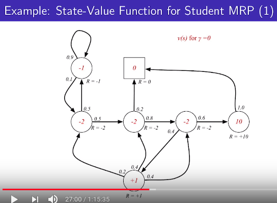
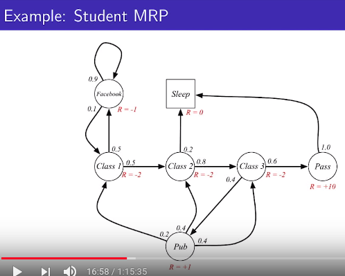 R is reward
================================================================================
RL is game which maximizes "return"
* Paths like "C1 C2 Pass..", "C1 F2 Pub..." can be sampled
* Return is summation of all rewards on each path, with using discount factor $$$\gamma$$$
* Formally, return $$$G_t$$$ is total discounted reward from time t
$$$G_t = R_{t+1}+\gamma R_{t+2}+\cdots=\sum\limits_{k=0}^{\infty}\gamma^k R_{t+k+1}$$$
* Goal of RL is to maximize cumulative discounted reward
================================================================================
R is reward
================================================================================
RL is game which maximizes "return"
* Paths like "C1 C2 Pass..", "C1 F2 Pub..." can be sampled
* Return is summation of all rewards on each path, with using discount factor $$$\gamma$$$
* Formally, return $$$G_t$$$ is total discounted reward from time t
$$$G_t = R_{t+1}+\gamma R_{t+2}+\cdots=\sum\limits_{k=0}^{\infty}\gamma^k R_{t+k+1}$$$
* Goal of RL is to maximize cumulative discounted reward
================================================================================
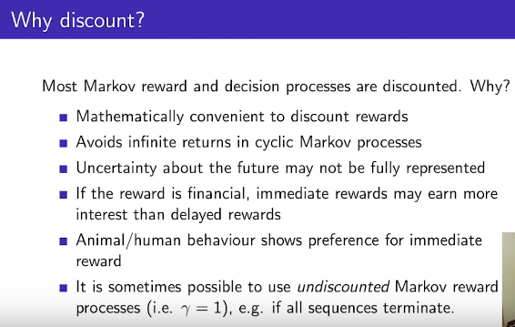 1. Mathematically convergence
================================================================================
1. Mathematically convergence
================================================================================
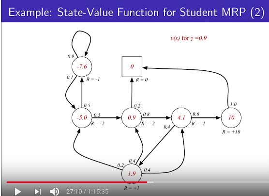
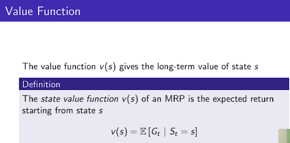 Value function
* Value function $$$v(s)$$$ is expectation value of return
expectation_val_of_return=value_function(state)
* Value function in MRP: $$$v(s)=\mathbb{E}[G_t|S_t=s]$$$
Value function in MDP has $$$\pi$$$ like $$$v_{\pi}(s)$$$
At s, agent samples paths along policy $$$\pi$$$, then, calculate expectation value of $$$G_t$$$
$$$G_t$$$: random variable
return_val1=Gt_random_variable(state1_path1)
return_val2=Gt_random_variable(state1_path2)
return_val3=Gt_random_variable(state1_path3)
expectation_val_of_return_val_at_state_1=value_function(return_val1,return_val2,return_val3)
* Value function $$$v(s)$$$ gives the "long-term value of state s"
================================================================================
Value function
* Value function $$$v(s)$$$ is expectation value of return
expectation_val_of_return=value_function(state)
* Value function in MRP: $$$v(s)=\mathbb{E}[G_t|S_t=s]$$$
Value function in MDP has $$$\pi$$$ like $$$v_{\pi}(s)$$$
At s, agent samples paths along policy $$$\pi$$$, then, calculate expectation value of $$$G_t$$$
$$$G_t$$$: random variable
return_val1=Gt_random_variable(state1_path1)
return_val2=Gt_random_variable(state1_path2)
return_val3=Gt_random_variable(state1_path3)
expectation_val_of_return_val_at_state_1=value_function(return_val1,return_val2,return_val3)
* Value function $$$v(s)$$$ gives the "long-term value of state s"
================================================================================
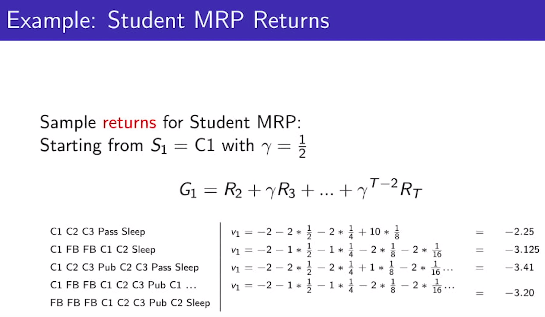 Sampled path1: C1 C2 C3 Pass Sleep
Start state: 1
Return value: -2.25
Sampled Path2: C1 FB FB C1 C2 Sleep
Start state: 1
Return value: -3.125
* Try to make average value: $$$-2.25+-3.125+\cdots$$$
* Agent can predict "return value" at state 1 (C1) based on average value
================================================================================
Sampled path1: C1 C2 C3 Pass Sleep
Start state: 1
Return value: -2.25
Sampled Path2: C1 FB FB C1 C2 Sleep
Start state: 1
Return value: -3.125
* Try to make average value: $$$-2.25+-3.125+\cdots$$$
* Agent can predict "return value" at state 1 (C1) based on average value
================================================================================
 ================================================================================
 ================================================================================
 ================================================================================
Bellman equation for MRPs
* Bellman equation is much used for value-based RL method
* Bellman equation controls value function
* value function is trained using iterative method and based on bellman equation
================================================================================
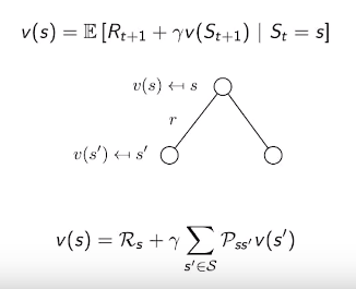
* value function can be decomposed into 2 parts
(1) immediate reward $$$R_{t+1}$$$ part
(2) discounted value of successor state $$$\gamma v(S_{t+1})$$$
================================================================================
* Definition of value function:
$$$v(s)=\mathbb{E}[G_t|S_t=s]$$$
* Spread $$$G_t=\mathbb{E}[R_{t+1}+\gamma R_{t+1} + \gamma^2 R_{t+3}+ \cdots | S_t=s]$$$
* Apply spread $$$G_t$$$
$$$v(s)=\mathbb{E}[R_{t+1}+\gamma R_{t+1} + \gamma^2 R_{t+3}+ \cdots|S_t=s]$$$
* Group by $$$\gamma$$$
$$$v(s)=\mathbb{E}[R_{t+1} + \gamma(R_{t+2} + \gamma R_{t+3} + \cdots) |S_t=s]$$$
* $$$R_{t+2} + \gamma R_{t+3} + \cdots = G_{t+1}$$$
* $$$v(s)=\mathbb{E}[R_{t+1} + \gamma v(S_{t+1}) |S_t=s]$$$
* Above shows relationship between $$$v(s)$$$ and $$$v(S_{t+1})$$$
================================================================================
================================================================================
Bellman equation for MRPs
* Bellman equation is much used for value-based RL method
* Bellman equation controls value function
* value function is trained using iterative method and based on bellman equation
================================================================================
* value function can be decomposed into 2 parts
(1) immediate reward $$$R_{t+1}$$$ part
(2) discounted value of successor state $$$\gamma v(S_{t+1})$$$
================================================================================
* Definition of value function:
$$$v(s)=\mathbb{E}[G_t|S_t=s]$$$
* Spread $$$G_t=\mathbb{E}[R_{t+1}+\gamma R_{t+1} + \gamma^2 R_{t+3}+ \cdots | S_t=s]$$$
* Apply spread $$$G_t$$$
$$$v(s)=\mathbb{E}[R_{t+1}+\gamma R_{t+1} + \gamma^2 R_{t+3}+ \cdots|S_t=s]$$$
* Group by $$$\gamma$$$
$$$v(s)=\mathbb{E}[R_{t+1} + \gamma(R_{t+2} + \gamma R_{t+3} + \cdots) |S_t=s]$$$
* $$$R_{t+2} + \gamma R_{t+3} + \cdots = G_{t+1}$$$
* $$$v(s)=\mathbb{E}[R_{t+1} + \gamma v(S_{t+1}) |S_t=s]$$$
* Above shows relationship between $$$v(s)$$$ and $$$v(S_{t+1})$$$
================================================================================
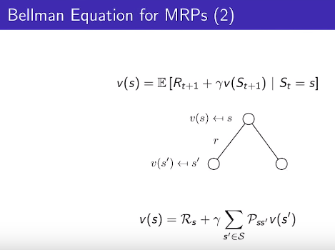
 Bellman equation: $$$v(s)=\mathbb{E}[R_{t+1} + \gamma v(S_{t+1}) |S_t=s]$$$
* Move from $$$s$$$ to $$$s^{'}$$$
* There are many ways to go from $$$s$$$ to $$$s^{'}$$$
like left circle and right circle
* For example, suppose probability $$$s$$$ to $$$s^{'}_{\text{left circle}}$$$ is 20%
probability $$$s$$$ to $$$s^{'}_{\text{right circle}}$$$ is 80%
Value of state s: $$$\mathcal{R}_s + \left[ 0.2\times s^{'}_{\text{left circle}} + 0.8\times s^{'}_{\text{right circle}} \right]$$$
$$$\mathcal{R}_s$$$: reward at state s
================================================================================
Bellman equation: $$$v(s)=\mathbb{E}[R_{t+1} + \gamma v(S_{t+1}) |S_t=s]$$$
* Move from $$$s$$$ to $$$s^{'}$$$
* There are many ways to go from $$$s$$$ to $$$s^{'}$$$
like left circle and right circle
* For example, suppose probability $$$s$$$ to $$$s^{'}_{\text{left circle}}$$$ is 20%
probability $$$s$$$ to $$$s^{'}_{\text{right circle}}$$$ is 80%
Value of state s: $$$\mathcal{R}_s + \left[ 0.2\times s^{'}_{\text{left circle}} + 0.8\times s^{'}_{\text{right circle}} \right]$$$
$$$\mathcal{R}_s$$$: reward at state s
================================================================================
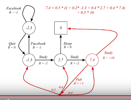
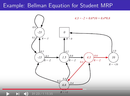 * See 4.3 circle
$$$-2 + \left[ 0.6\times 10 + 0.4\times 0.8 \right]$$$
-2: $$$R_s$$$
* Bellman equation value:
(1) you can get solution directly in MRP
(2) you can get solution using iterative method in MDP
================================================================================
Let's express following equation
* See 4.3 circle
$$$-2 + \left[ 0.6\times 10 + 0.4\times 0.8 \right]$$$
-2: $$$R_s$$$
* Bellman equation value:
(1) you can get solution directly in MRP
(2) you can get solution using iterative method in MDP
================================================================================
Let's express following equation
 into vector and matrix
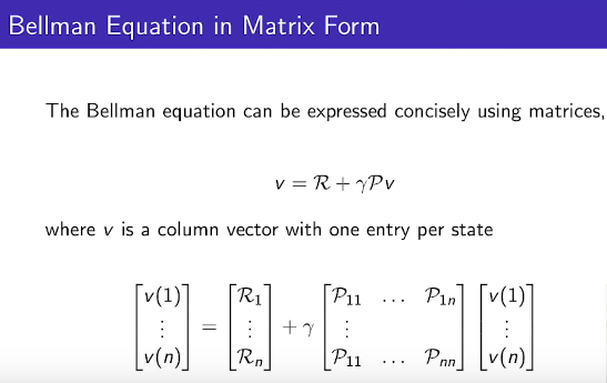 * Bellman equation is a linear equation
* v vector
* R vector
* P transition matrix
================================================================================
* Bellman equation is a linear equation
* v vector
* R vector
* P transition matrix
================================================================================
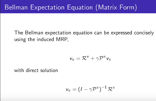
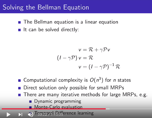 * Meaning: when you're given $$$\mathcal{R},\mathcal{P},\gamma$$$ which are definition of MRP
value function can be found directly by calculating $$$v=(\mathcal{I}-\gamma \mathcal{P})^{-1} \mathcal{R}$$$
* Computational complexity is O(n^3) for n number of states
Quite high computational when you have many state
* So, it's direct solution for small MRPs
* You can use iterative methods for large MRP
(1) Dynamic programming
(2) Monte Carlo evaluation
which is similar to Monte Carlo tree but they're not identical.
(3) Temporal Difference learnign
================================================================================
Markov decision process
* Definition: $$$\langle \mathcal{S},\mathcal{A},\mathcal{P},\mathcal{R},\gamma \rangle$$$
MDP = MP + A,R,$$$\gamma$$$
MDP = MRP + A
* $$$\mathcal{S}$$$: finite set of states
* $$$\mathcal{A}$$$: finite set of actions
* $$$\mathcal{P}$$$: state transition probability matrix
$$$\mathcal{P}_{ss^{'}}^a = \mathbb{P} [S_{t+1}=s^{'}| S_t=s,A_t=a]$$$
* $$$\mathcal{R}$$$ is reward function
$$$\mathcal{R}_s^a = \mathbb{E} [R_{t+1} | S_t=s,A_t=a]$$$
* All states are markov states
================================================================================
* Meaning: when you're given $$$\mathcal{R},\mathcal{P},\gamma$$$ which are definition of MRP
value function can be found directly by calculating $$$v=(\mathcal{I}-\gamma \mathcal{P})^{-1} \mathcal{R}$$$
* Computational complexity is O(n^3) for n number of states
Quite high computational when you have many state
* So, it's direct solution for small MRPs
* You can use iterative methods for large MRP
(1) Dynamic programming
(2) Monte Carlo evaluation
which is similar to Monte Carlo tree but they're not identical.
(3) Temporal Difference learnign
================================================================================
Markov decision process
* Definition: $$$\langle \mathcal{S},\mathcal{A},\mathcal{P},\mathcal{R},\gamma \rangle$$$
MDP = MP + A,R,$$$\gamma$$$
MDP = MRP + A
* $$$\mathcal{S}$$$: finite set of states
* $$$\mathcal{A}$$$: finite set of actions
* $$$\mathcal{P}$$$: state transition probability matrix
$$$\mathcal{P}_{ss^{'}}^a = \mathbb{P} [S_{t+1}=s^{'}| S_t=s,A_t=a]$$$
* $$$\mathcal{R}$$$ is reward function
$$$\mathcal{R}_s^a = \mathbb{E} [R_{t+1} | S_t=s,A_t=a]$$$
* All states are markov states
================================================================================
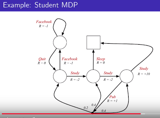
 * Name of states is not important. So they're void.
* Study: action of study
* MRP has reward at each state
* MDP has reward at each action
* When agent does "action", agent doesn't directly go to specific state
When agent does "action", agent goes to specific state in some probabilities which each action has
* See center and right circles
Agent goes from center circle to right circle in 1.0 probability which Study has
================================================================================
* Name of states is not important. So they're void.
* Study: action of study
* MRP has reward at each state
* MDP has reward at each action
* When agent does "action", agent doesn't directly go to specific state
When agent does "action", agent goes to specific state in some probabilities which each action has
* See center and right circles
Agent goes from center circle to right circle in 1.0 probability which Study has
================================================================================
 $$$\mathcal{P}_{ss^{'}}$$$ in MRP: probability of going from $$$s$$$ to $$$s^{'}$$$
$$$\mathcal{P}$$$ is $$$m\times m$$$ matrix
================================================================================
$$$\mathcal{P}_{ss^{'}}$$$ in MRP: probability of going from $$$s$$$ to $$$s^{'}$$$
$$$\mathcal{P}$$$ is $$$m\times m$$$ matrix
================================================================================
 * Note that there is a in superscript
* $$$\mathcal{P}_{ss^{'}}^a$$$: probability of going from $$$s$$$ to $$$s^{'}$$$
when agent does action a at state s
* comparison
(1) In MRP, probability of going from $$$s$$$ to $$$s^{'}$$$
(2) In MDP, probabilities of going from $$$s$$$ to $$$s^{'}$$$
when agent does each action a at state s
action1 to go from $$$s$$$ to $$$s^{'}$$$: prob1
action2 to go from $$$s$$$ to $$$s^{'}$$$: prob2
action3 to go from $$$s$$$ to $$$s^{'}$$$: prob3
================================================================================
* In MRP, there is no policy, because agent doesn't do action.
* In MRP, agent automatically moves from s to s^{'} based on transition state probability
================================================================================
* In MDP, agent does action.
* Along chosen action, next states vary.
* So, choosing action based on policy is important
================================================================================
* Note that there is a in superscript
* $$$\mathcal{P}_{ss^{'}}^a$$$: probability of going from $$$s$$$ to $$$s^{'}$$$
when agent does action a at state s
* comparison
(1) In MRP, probability of going from $$$s$$$ to $$$s^{'}$$$
(2) In MDP, probabilities of going from $$$s$$$ to $$$s^{'}$$$
when agent does each action a at state s
action1 to go from $$$s$$$ to $$$s^{'}$$$: prob1
action2 to go from $$$s$$$ to $$$s^{'}$$$: prob2
action3 to go from $$$s$$$ to $$$s^{'}$$$: prob3
================================================================================
* In MRP, there is no policy, because agent doesn't do action.
* In MRP, agent automatically moves from s to s^{'} based on transition state probability
================================================================================
* In MDP, agent does action.
* Along chosen action, next states vary.
* So, choosing action based on policy is important
================================================================================
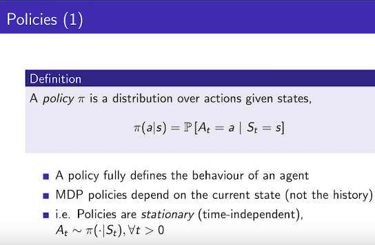 * Definition of policy $$$\pi$$$
$$$\pi(a|s) = \mathbb{P} [A_t=a | S_t=s]$$$
At state s, probability of doing action a
* Policy determines action of agent
* MDP policies depend on only "current state" (not the history)
If agent has current state, agent determines decision
because agent is in MDP (fully observable environment)
================================================================================
* Definition of policy $$$\pi$$$
$$$\pi(a|s) = \mathbb{P} [A_t=a | S_t=s]$$$
At state s, probability of doing action a
* Policy determines action of agent
* MDP policies depend on only "current state" (not the history)
If agent has current state, agent determines decision
because agent is in MDP (fully observable environment)
================================================================================
 * You can't see policy from above illustration
* Above illustration is MDP (environment)
* Policy is owned by "agent"
* Agent says "I'll move MDP environment using policies at each state"
There can be multiple policies.
What policy will make sum of reward which agent will have?
Above sentence is the goal of solving MDP.
================================================================================
* You can't see policy from above illustration
* Above illustration is MDP (environment)
* Policy is owned by "agent"
* Agent says "I'll move MDP environment using policies at each state"
There can be multiple policies.
What policy will make sum of reward which agent will have?
Above sentence is the goal of solving MDP.
================================================================================
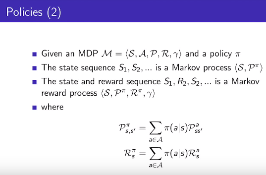 * Suppose agent moves based on policy $$$\pi$$$ in MDP
* Agent visits states
states have multiple cadidate actions
Agent choose one action based on policy
Chosen action has "state transition" so that agent moves to next state
* You can group above conditions to consider MPD as MP (which has only S and P)
* But constraints are that MDP and $$$\pi$$$ should be fixed
Then, at specific state, you can manually calculate all probabilieis of next state
* How to calculate those probabilieis?
(1) $$$\mathcal{P}_{s,s^{'}}^{\pi} = \sum\limits_{a\in \mathcal{A}} \pi(a|s) \mathcal{P}_{ss^{'}}^a$$$
$$$\mathcal{P}_{s,s^{'}}^\pi$$$: probability of agent going from $$$s$$$ to $$$s^{'}$$$ based on policy $$$\pi$$$
$$$\pi(a|s)$$$: probability of agent doing action a at state s
$$$\mathcal{P}_{s,s^{'}}^a$$$: probability of agent going from $$$s$$$ to $$$s^{'}$$$
when agent does action a
$$$\sum\limits_{a\in \mathcal{A}}$$$: sum all action cases
(2) $$$\mathcal{R}_{s}^\pi = \sum\limits_{a \in \mathcal{A}} \pi(a|s) \mathcal{R}_{s}^a$$$
================================================================================
State and reward sequence ($$$S_1,R_2,S_2,\cdots$$$) becomes Markov reward process $$$\langle \mathcal{S},\mathcal{P}^{\pi},\mathcal{R}^{\pi},\gamma \rangle$$$
$$$\mathcal{R}_{s}^{\pi} = \sum\limits_{a\in \mathcal{A}} \pi(a|s) \mathcal{R}_s^a$$$
================================================================================
* Suppose agent moves based on policy $$$\pi$$$ in MDP
* Agent visits states
states have multiple cadidate actions
Agent choose one action based on policy
Chosen action has "state transition" so that agent moves to next state
* You can group above conditions to consider MPD as MP (which has only S and P)
* But constraints are that MDP and $$$\pi$$$ should be fixed
Then, at specific state, you can manually calculate all probabilieis of next state
* How to calculate those probabilieis?
(1) $$$\mathcal{P}_{s,s^{'}}^{\pi} = \sum\limits_{a\in \mathcal{A}} \pi(a|s) \mathcal{P}_{ss^{'}}^a$$$
$$$\mathcal{P}_{s,s^{'}}^\pi$$$: probability of agent going from $$$s$$$ to $$$s^{'}$$$ based on policy $$$\pi$$$
$$$\pi(a|s)$$$: probability of agent doing action a at state s
$$$\mathcal{P}_{s,s^{'}}^a$$$: probability of agent going from $$$s$$$ to $$$s^{'}$$$
when agent does action a
$$$\sum\limits_{a\in \mathcal{A}}$$$: sum all action cases
(2) $$$\mathcal{R}_{s}^\pi = \sum\limits_{a \in \mathcal{A}} \pi(a|s) \mathcal{R}_{s}^a$$$
================================================================================
State and reward sequence ($$$S_1,R_2,S_2,\cdots$$$) becomes Markov reward process $$$\langle \mathcal{S},\mathcal{P}^{\pi},\mathcal{R}^{\pi},\gamma \rangle$$$
$$$\mathcal{R}_{s}^{\pi} = \sum\limits_{a\in \mathcal{A}} \pi(a|s) \mathcal{R}_s^a$$$
================================================================================
 * Value function in MRP doesn't have $$$\pi$$$
because agent doesn't do action
* Value function in MDP have $$$\pi$$$ to define value function
$$$v_\pi(s) = \mathbb{E}_\pi [G_t|S_t=s]$$$
* At state s, agent plays game until the end of game, following a policy
it creates one episode
* You do sampling many episodes
* You perform average samepled episodes, and it's value functionn
================================================================================
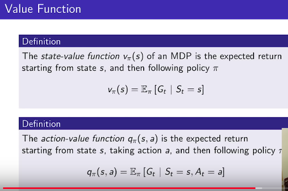
There are 2 value functions in MDP
(1) state value action
* $$$v_\pi(s) = \mathbb{E}_\pi [G_t|S_t=s]$$$
* expectation_val_of_all_return_vals_G_t=state_value_function(state)
(2) action value fucntion (aka Q function which is target of training in DQN)
* $$$q_\pi(s,a) = \mathbb{E}_\pi [G_t|S_t=s,A_t=a]$$$
* expectation_val_of_all_return_vals_G_t=action_value_function(state,action)
* At state s, agent does action a, after that action,
agent plays the game until the end of game by following policy $$$\pi$$$
you calculate expectation value of return values
================================================================================
* You will express relationship between state value function and action-value function
by using bellman equation
* When solving large problem, bellman equation is base algorithm
================================================================================
* Value function in MRP doesn't have $$$\pi$$$
because agent doesn't do action
* Value function in MDP have $$$\pi$$$ to define value function
$$$v_\pi(s) = \mathbb{E}_\pi [G_t|S_t=s]$$$
* At state s, agent plays game until the end of game, following a policy
it creates one episode
* You do sampling many episodes
* You perform average samepled episodes, and it's value functionn
================================================================================
There are 2 value functions in MDP
(1) state value action
* $$$v_\pi(s) = \mathbb{E}_\pi [G_t|S_t=s]$$$
* expectation_val_of_all_return_vals_G_t=state_value_function(state)
(2) action value fucntion (aka Q function which is target of training in DQN)
* $$$q_\pi(s,a) = \mathbb{E}_\pi [G_t|S_t=s,A_t=a]$$$
* expectation_val_of_all_return_vals_G_t=action_value_function(state,action)
* At state s, agent does action a, after that action,
agent plays the game until the end of game by following policy $$$\pi$$$
you calculate expectation value of return values
================================================================================
* You will express relationship between state value function and action-value function
by using bellman equation
* When solving large problem, bellman equation is base algorithm
================================================================================
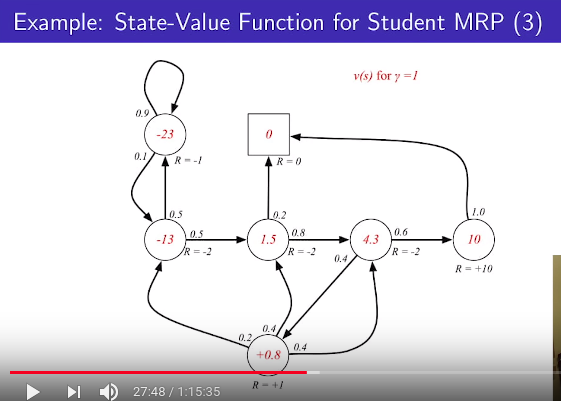
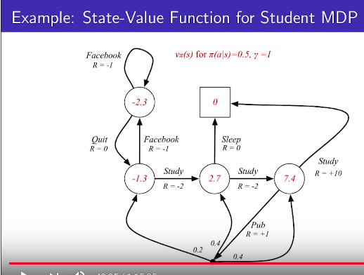 Policy: at all states, each action has 0.5 probability
$$$\pi(a|s)=0.5$$$
* When agent follow above policy, red numbers are calculated state-value function
================================================================================
Policy: at all states, each action has 0.5 probability
$$$\pi(a|s)=0.5$$$
* When agent follow above policy, red numbers are calculated state-value function
================================================================================
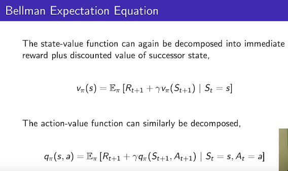 (1) Bellman expectation equation
(2) Bellman optimility equation
Let's see Bellman expectation equation
* State-value function can be decomposed
into "immediate reward" and "discounted value of successor state"
$$$v_\pi(s) = \mathbb{E}_{\pi}[R_{t+1} + \gamma v_{\pi}(S_{t+1}) | S_t=s]$$$
- Meaning
(1) Go one step
(2) After that step, agent goes along policy
(3) expectation of (1)(2) = state-value function
* Action-value function can be decomposed into
$$$q_{\pi}(s,a) = \mathbb{E}_{\pi}[R_{t+1} + \gamma q_{\pi}(S_{t+1},A_{t+1}) | S_t=s,A_t=a]$$$
(1) Agent does action a at state s
(2) Agent gets reward
(3) At next state, agent does next action
(4) expectation of (1)(2)(3) = action-value function
================================================================================
(1) Bellman expectation equation
(2) Bellman optimility equation
Let's see Bellman expectation equation
* State-value function can be decomposed
into "immediate reward" and "discounted value of successor state"
$$$v_\pi(s) = \mathbb{E}_{\pi}[R_{t+1} + \gamma v_{\pi}(S_{t+1}) | S_t=s]$$$
- Meaning
(1) Go one step
(2) After that step, agent goes along policy
(3) expectation of (1)(2) = state-value function
* Action-value function can be decomposed into
$$$q_{\pi}(s,a) = \mathbb{E}_{\pi}[R_{t+1} + \gamma q_{\pi}(S_{t+1},A_{t+1}) | S_t=s,A_t=a]$$$
(1) Agent does action a at state s
(2) Agent gets reward
(3) At next state, agent does next action
(4) expectation of (1)(2)(3) = action-value function
================================================================================
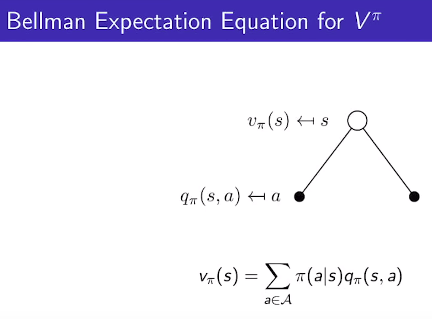 You can express v by using q
$$$v_\pi(s)=\sum\limits_{a\in \\mathcal{A}} \pi(a|s)q_{\pi}(s,a)$$$
================================================================================
You can express v by using q
$$$v_\pi(s)=\sum\limits_{a\in \\mathcal{A}} \pi(a|s)q_{\pi}(s,a)$$$
================================================================================
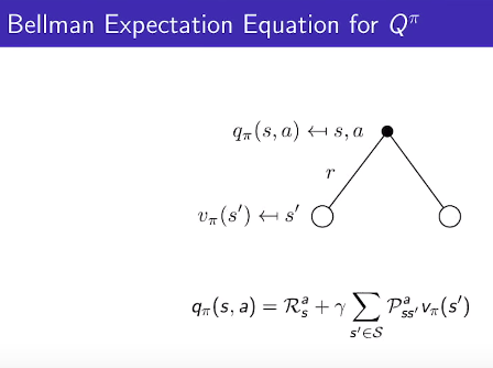 You can express q by using v
$$$q_{\pi}(s,a) = \mathcal{R}_{s}^{a} + \gamma \sum\limits_{s^{'}\in \mathcal{S}} \mathcal{P}_{ss^{'}}^{a} v_\pi(s^{'})$$$
================================================================================
You can express q by using v
$$$q_{\pi}(s,a) = \mathcal{R}_{s}^{a} + \gamma \sum\limits_{s^{'}\in \mathcal{S}} \mathcal{P}_{ss^{'}}^{a} v_\pi(s^{'})$$$
================================================================================
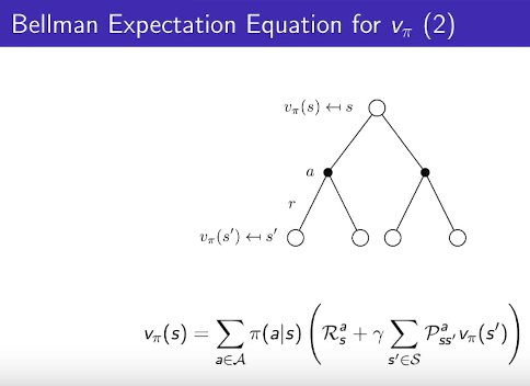 You use 1 and 2 to express $$$v_{\pi}(s)$$$
================================================================================
You use 1 and 2 to express $$$v_{\pi}(s)$$$
================================================================================
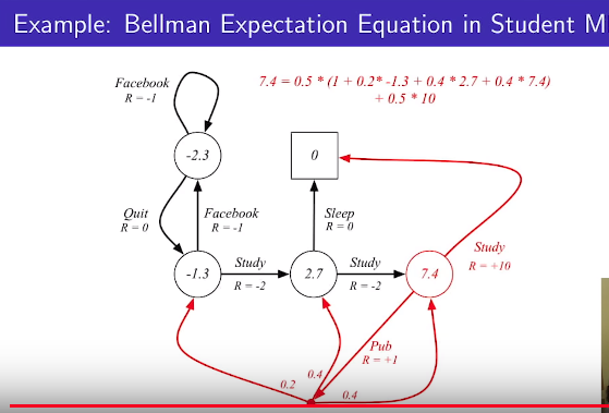 Example: Bellman Expectation Equation in Student MDP using above equation
policy $$$\pi(a|s)=0.5$$$
================================================================================
Example: Bellman Expectation Equation in Student MDP using above equation
policy $$$\pi(a|s)=0.5$$$
================================================================================
 ================================================================================
You can solve value function in MDP by using Bellman equation
$$$v_\pi$$$ means value when agent does action with following policy $$$\pi$$$
Again, value can be calculated like this when $$$\pi(a|s)=0.5$$$
================================================================================
You can solve value function in MDP by using Bellman equation
$$$v_\pi$$$ means value when agent does action with following policy $$$\pi$$$
Again, value can be calculated like this when $$$\pi(a|s)=0.5$$$
 ================================================================================
 Goal is to find optimal value function
* So far, you suppose there is policy $$$\pi$$$
But fixed $$$\pi$$$=0.5 can be bad because it's 50%:50%
In that policy, you could find value function by using Bellman expectation equation
* When you find optimal value function, you should use Bellman optimility equation
================================================================================
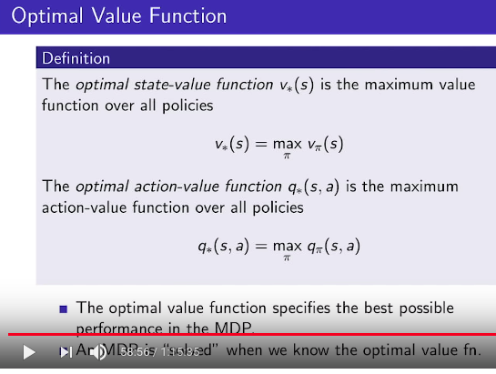
Definition of optimal state-value function $$$v_{*}(s)$$$
* $$$\pi$$$: certain policy \pi which agent follows
* $$$*$$$: there are many policies which agent can follow.
* There are many values cause there are many policies
* From those many values, best value is optimal value function
* optimal state-value function $$$v_{*}(s)$$$ is the maximum value function over "all policies"
* $$$v_{*}(s)=\max_{\pi} v_{\pi}(s)$$$
* There are many value functions which are determined by many policies $$$\pi$$$
* $$$\max_{\pi} v_{\pi}(s)$$$: From many value function, best value function
================================================================================
Definition of optimal action-value function q_{*}(s,a)
* Maximum action-value function over all policies
* $$$q_{*}(s,a) = \max_{\pi} q_{\pi}(s,a)$$$
* There are many q functions which follows polici $$$\pi$$$
From those many q functions, find max q
================================================================================
* Optimal value function shows best possible performance in MDP
* You can say MDP is "solved" when you can know the optimal value function.
================================================================================
Goal is to find optimal value function
* So far, you suppose there is policy $$$\pi$$$
But fixed $$$\pi$$$=0.5 can be bad because it's 50%:50%
In that policy, you could find value function by using Bellman expectation equation
* When you find optimal value function, you should use Bellman optimility equation
================================================================================
Definition of optimal state-value function $$$v_{*}(s)$$$
* $$$\pi$$$: certain policy \pi which agent follows
* $$$*$$$: there are many policies which agent can follow.
* There are many values cause there are many policies
* From those many values, best value is optimal value function
* optimal state-value function $$$v_{*}(s)$$$ is the maximum value function over "all policies"
* $$$v_{*}(s)=\max_{\pi} v_{\pi}(s)$$$
* There are many value functions which are determined by many policies $$$\pi$$$
* $$$\max_{\pi} v_{\pi}(s)$$$: From many value function, best value function
================================================================================
Definition of optimal action-value function q_{*}(s,a)
* Maximum action-value function over all policies
* $$$q_{*}(s,a) = \max_{\pi} q_{\pi}(s,a)$$$
* There are many q functions which follows polici $$$\pi$$$
From those many q functions, find max q
================================================================================
* Optimal value function shows best possible performance in MDP
* You can say MDP is "solved" when you can know the optimal value function.
================================================================================
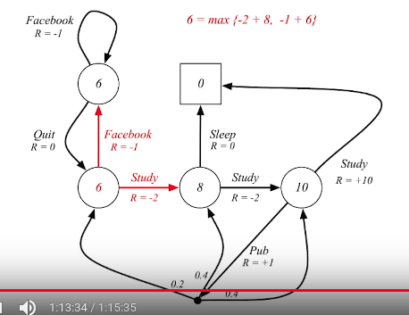
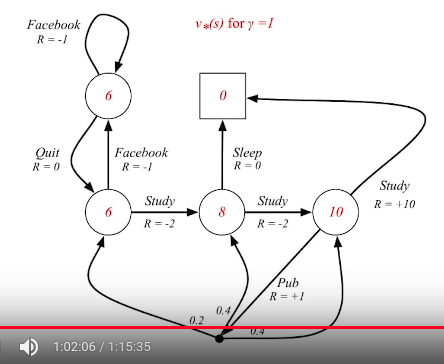 Above shows optimal value function when $$$\gamma=1$$$ in student MDP
Red numbers are optimal values
================================================================================
Above shows optimal value function when $$$\gamma=1$$$ in student MDP
Red numbers are optimal values
================================================================================
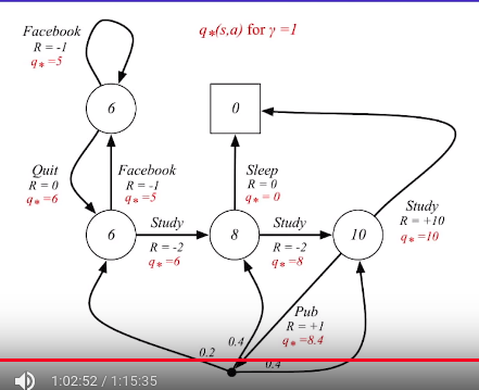 Optimal action-value function when $$$\gamma=1$$$ in student MDP
================================================================================
Optimal policy
To define optimal policy, you should be able to compare 2 policies
Comparison can be perform by using "partial ordering"
$$$\pi \ge \pi^{'}$$$ if $$$v_{\pi}(s) \ge v_{\pi^{'}}(s)$$$, $$$\forall s$$$
================================================================================
And there is theorem
* For any MDP
* $$$\pi_{*} \ge \pi$$$, $$$\forall \pi$$$
There exists an optimal policy $$$\pi$$$
that is better than or equal to all other policies
* $$$v_{\pi_*}(s) = v_{*}(s)$$$
All optimal policies achieve the optimal value function
* $$$q_{\pi_*}(s,a) = q_{*}(s,a)$$$
All optimal policies achieve the optimal action-value function
* Optimal policies can be multiple
================================================================================
As soon as you can find $$$q_*(s,a)$$$, you find optimal policy
$$$q_*(s,a)$$$: at state s, what action should agent do based on q value
================================================================================
Optimal policy can be found by maximizing over q_{*}(s,a)
Suppose policy is like
$$$\pi_{*}(a|s) = 1$$$ if $$$a = \arg_{a\in \mathcal{A}} \max q_{*}(s,a)$$$
at state s, when agent knows $$$q_*$$$, probability of agent doing action of $$$q_{*}$$$ is 1
$$$\pi_{*}(a|s) = 0$$$ otherwise
- Meaning: if agent knows optimal q, if agent follows optimal q,
agent is supposed to follow optimal policy
================================================================================
In MDP, policy is basically stochastic policy
because poilcy defines probabilieis on each action
But if one probability is 1 and others are 0s,
it becomes deterministic policy
So, you can say "there should be deterministic optimal policy for any MDP"
================================================================================
Optimal policy for student MDP
Optimal action-value function when $$$\gamma=1$$$ in student MDP
================================================================================
Optimal policy
To define optimal policy, you should be able to compare 2 policies
Comparison can be perform by using "partial ordering"
$$$\pi \ge \pi^{'}$$$ if $$$v_{\pi}(s) \ge v_{\pi^{'}}(s)$$$, $$$\forall s$$$
================================================================================
And there is theorem
* For any MDP
* $$$\pi_{*} \ge \pi$$$, $$$\forall \pi$$$
There exists an optimal policy $$$\pi$$$
that is better than or equal to all other policies
* $$$v_{\pi_*}(s) = v_{*}(s)$$$
All optimal policies achieve the optimal value function
* $$$q_{\pi_*}(s,a) = q_{*}(s,a)$$$
All optimal policies achieve the optimal action-value function
* Optimal policies can be multiple
================================================================================
As soon as you can find $$$q_*(s,a)$$$, you find optimal policy
$$$q_*(s,a)$$$: at state s, what action should agent do based on q value
================================================================================
Optimal policy can be found by maximizing over q_{*}(s,a)
Suppose policy is like
$$$\pi_{*}(a|s) = 1$$$ if $$$a = \arg_{a\in \mathcal{A}} \max q_{*}(s,a)$$$
at state s, when agent knows $$$q_*$$$, probability of agent doing action of $$$q_{*}$$$ is 1
$$$\pi_{*}(a|s) = 0$$$ otherwise
- Meaning: if agent knows optimal q, if agent follows optimal q,
agent is supposed to follow optimal policy
================================================================================
In MDP, policy is basically stochastic policy
because poilcy defines probabilieis on each action
But if one probability is 1 and others are 0s,
it becomes deterministic policy
So, you can say "there should be deterministic optimal policy for any MDP"
================================================================================
Optimal policy for student MDP
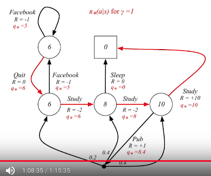 Red arrows consist of optimal policy
================================================================================
Red arrows consist of optimal policy
================================================================================
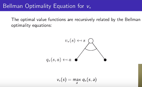
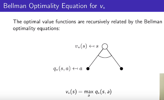 To find optimal value at state $$$s$$$,
you should choose max from $$$q^{*}(s,a)$$$
$$$v_{*}(s) \max_{a} q_{*}(s,a)$$$
$$$q_{*}$$$ values are owned by each action a
From those, select $$$\max_{a} q_{*}(s,a)$$$
If agent does this, it becomes what action a chooses is v
================================================================================
To find optimal value at state $$$s$$$,
you should choose max from $$$q^{*}(s,a)$$$
$$$v_{*}(s) \max_{a} q_{*}(s,a)$$$
$$$q_{*}$$$ values are owned by each action a
From those, select $$$\max_{a} q_{*}(s,a)$$$
If agent does this, it becomes what action a chooses is v
================================================================================
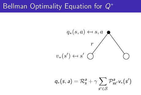 Let's express Q by using v
================================================================================
Let's express Q by using v
================================================================================
 Let's express v by using q
================================================================================
Merge them.
Let's express v by using q
================================================================================
Merge them.
 $$$v_{*}(s) = \max_{a} \left[ \mathcal{R}_{s}^{a} + \gamma \sum\limits_{s^{'}\in \mathcal{S}} \mathcal{P}_{ss^{'}}^{a} v_{*}(s^{'})\right]$$$
Above one is not linear equation. So it can't be solved by closed form method
================================================================================
Bellman optimality equation in student MDP
$$$v_{*}(s) = \max_{a} \left[ \mathcal{R}_{s}^{a} + \gamma \sum\limits_{s^{'}\in \mathcal{S}} \mathcal{P}_{ss^{'}}^{a} v_{*}(s^{'})\right]$$$
Above one is not linear equation. So it can't be solved by closed form method
================================================================================
Bellman optimality equation in student MDP
 ================================================================================
Methods to solve bellman optimality equation
* Bellman optimality equation is non-linear
* So, there is no closed form solution (in general)
* So, there are many iterative solution methods.
(1) Value iteration (Dymanic programming methodology)
(2) Policy iteration (Dymanic programming methodology)
(3) Q-learning
(4) SARSA
================================================================================
Methods to solve bellman optimality equation
* Bellman optimality equation is non-linear
* So, there is no closed form solution (in general)
* So, there are many iterative solution methods.
(1) Value iteration (Dymanic programming methodology)
(2) Policy iteration (Dymanic programming methodology)
(3) Q-learning
(4) SARSA