https://www.youtube.com/watch?v=rrTxOkbHj-M
================================================================================
Planning
- When agent knows all information about MDP (environment, state)
planning is to find optimal policy
- Method for planning
Dynamic programming
================================================================================
Outline
* Introduction
* Policy evaluation
* Policy iteration
* value iteration
* extensions to dynamic programming
* contraction mapping
================================================================================
Policy evaluation
* When policy is determined, if agent goes along the policy in MDP,
policy evaluation is to find value function
* policy is fixed, find value function
================================================================================
Use following iterative methods to find optimal policy
* Policy iteration: policy based method
* Value iteration: value based method
================================================================================
Dynamic programming
* It's a methodology to solve complicated problem.
* You break large problem into small sub problems.
* You find solutions on each small sub problem.
* And you gather those solutions to find solution for large problem.
================================================================================
Reinforcement learning: model free, model based
* model free: agent doesn't know what he will get from environment
* model based: agent has environment model
"do some action, agent arrives at some state with some probability" are known
* Planning is used for model based reinforcement learning
* To solve planning, dynamic programming is used.
================================================================================
Requirements for dynamic programming
* Optimal substructure
Optimal solution of large problem should be able to be devided into small problems.
* Subproblems should be overwrapped
If you solve a subproblem, that subproblem should recur many times in various places.
So, you need to store solution of that subproblem in the form of cache to reuse it.
================================================================================
Markov decision processes (MDP) satisfy above 2 requirements.
* Optimal substructure
* Subproblems should be overwrapped
================================================================================
Dynamic programming assumes following full knowledge of the MDP
state transition probability, reward, etc
Dynamic programming is used for planning in an MDP (when agent know model)
to find optimal policy
================================================================================
Solve planning
* Solve prediction
1. Solve prediction learns value function
2. Given input: MDP $$$\langle \mathcal{S},\mathcal{A},\mathcal{P},\mathcal{R},\gamma \rangle$$$ and policy $$$\pi$$$
You can be given MRP $$$\langle \mathcal{S},\mathcal{P}^{\pi},\mathcal{R}^{\pi},\gamma \rangle$$$ instead of MDP
3. Output: you would like to find value function $$$v_{\pi}$$$
as you follow known policy $$$\pi$$$
4. "Solving prediction" is nothing to do with optimal policy.
No matter how bad optimal policy is given, agent follows that policy in MDP,
you predict return up to end point via value function
* Solve control
1. Solve control learns optimal policy
2. Given input: MDP $$$\langle \mathcal{S},\mathcal{A},\mathcal{P},\mathcal{R},\gamma \rangle$$$
3. Output: you would like to find optimal value function $$$v_{\pi}$$$
and optimal policy $$$\pi_{*}$$$
================================================================================
To define MDP, you need 5 components
* $$$\mathcal{S}$$$: set of states
* $$$\mathcal{A}$$$: set of actions
* $$$\mathcal{P}$$$: transition matrix, when agent does action a at state s,
probabilities of next states, which are written in matrix
* $$$\mathcal{R}$$$: set of rewards
* $$$\gamma$$$: discount factor
================================================================================
Dynamic programing is much used for other domains
* Scheduling algorithm
* String algorithm (e.g., sequence alignment)
* Graph algorithm (e.g., shortest path algorithm)
* Graphical models (e.g., viterbi algorithm)
* Bioinformatics (e.g., lattice models)
* Planning
================================================================================
Policy evaluation
* It's problem of evaluating policy.
* Evaluating policy means what's "return value" when agent follows the "policy"
High return means good evaluated policy.
* Since return value is returned from value function, you need to find value function.
================================================================================
How to solve policy evaluation
* you iteratively use Bellman expectation equation
1. set random v, meaning values at all states are 0, which is $$$v_1$$$
2. use iterative method and get $$$v_2$$$
3. your goal is to converge $$$v$$$ into $$$v_{\pi}$$$ which is function wrt policy $$$\pi$$$
4. Use synchronous backups
(1)
================================================================================
Bellman expectation equation
 - Iterative form: k+1 and k are grouped in one equation
Express v by q, express q by v, insert v into q, then, you can express v by v
- By using this, you can update all values per iteration
- $$$v_{k+1}(s) \leftarrow s$$$: state s, you get value $$$v_{k+1}(s)$$$ at k+1 time
- You goal is to make value more precise at k+1
- At k+1, you have 4 states agent can go.
- You use 4 states and you update value at k+1
- At initial time, 4 states has garbage random values
- By updating many times, they become precise
- Why it works? states are garbage, but reward is fixed and precise value
So, fixed and precise known value is inserted into that iteration,
so you will get precise values in the end.
================================================================================
- Iterative form: k+1 and k are grouped in one equation
Express v by q, express q by v, insert v into q, then, you can express v by v
- By using this, you can update all values per iteration
- $$$v_{k+1}(s) \leftarrow s$$$: state s, you get value $$$v_{k+1}(s)$$$ at k+1 time
- You goal is to make value more precise at k+1
- At k+1, you have 4 states agent can go.
- You use 4 states and you update value at k+1
- At initial time, 4 states has garbage random values
- By updating many times, they become precise
- Why it works? states are garbage, but reward is fixed and precise value
So, fixed and precise known value is inserted into that iteration,
so you will get precise values in the end.
================================================================================
 Evaluating a random policy in the small gridworld
- Prediction problem: so you are given MDP and policy $$$\pi$$$
- (4,4) matrix is MDP
- States 16 (including 2 terminal states)
- You have 4 actions at each state
- Policy is random, so each action has $$$\frac{1}{4}$$$ probability
================================================================================
Evaluating a random policy in the small gridworld
- Prediction problem: so you are given MDP and policy $$$\pi$$$
- (4,4) matrix is MDP
- States 16 (including 2 terminal states)
- You have 4 actions at each state
- Policy is random, so each action has $$$\frac{1}{4}$$$ probability
================================================================================
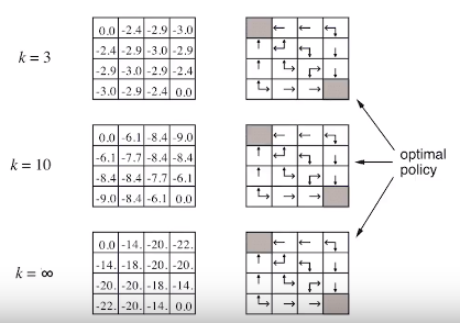
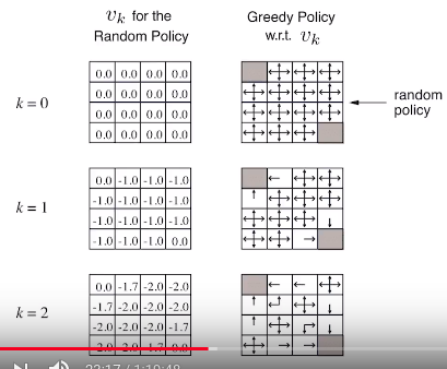 $$$v_k$$$ is initialized by 0 for the "random policy"
Right illustratioins represente policy
After you update values by using above Bellman exprectation equation,
you get illustratioins at k=1
================================================================================
$$$v_k$$$ is initialized by 0 for the "random policy"
Right illustratioins represente policy
After you update values by using above Bellman exprectation equation,
you get illustratioins at k=1
================================================================================
 ================================================================================
Policy iteration
================================================================================
Policy iteration
 1. You evaluate (bad) policy $$$\pi$$$
Evaluating policy means you find value function
2. You newly create policy which greedly moves (agent moves along highest value)
wrt that value function you're evaluating
3. You iterate "evaluate" and "improve"
================================================================================
1. You evaluate (bad) policy $$$\pi$$$
Evaluating policy means you find value function
2. You newly create policy which greedly moves (agent moves along highest value)
wrt that value function you're evaluating
3. You iterate "evaluate" and "improve"
================================================================================
 - Starting V_{\pi}: bad value function
$$$\pi$$$: bad policy
- First arrow: first evaluating value function $$$v_{\pi}$$$
And you get new value function
- Based on new value function, you get new policy $$$\pi$$$
by using $$$\pi=\text{greedy}(V)$$$
- You evaluate $$$\pi$$$
And you get new value function using $$$V^{\pi}=V_{\text{new}}$$$
- You use $$$\pi=\text{greedy}(V)$$$ again
- Finally, you get optial value function $$$v^{*}$$$ and optimal policy $$$\pi^{*}$$$
- Policy iteration: evaluation, improvement, evaluation, improvement, ...
================================================================================
Jack's Car Rental
- Starting V_{\pi}: bad value function
$$$\pi$$$: bad policy
- First arrow: first evaluating value function $$$v_{\pi}$$$
And you get new value function
- Based on new value function, you get new policy $$$\pi$$$
by using $$$\pi=\text{greedy}(V)$$$
- You evaluate $$$\pi$$$
And you get new value function using $$$V^{\pi}=V_{\text{new}}$$$
- You use $$$\pi=\text{greedy}(V)$$$ again
- Finally, you get optial value function $$$v^{*}$$$ and optimal policy $$$\pi^{*}$$$
- Policy iteration: evaluation, improvement, evaluation, improvement, ...
================================================================================
Jack's Car Rental
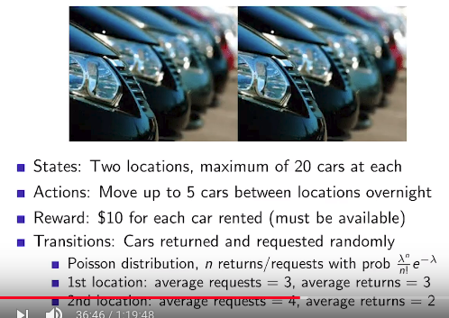 - States: there are 2 locations. 20 cars can be located at each location in maximum
- Action: move up to 5 cars between locations overnight.
- Transition:
1. Customers come to A location in Poisson distribution
Poisson distribution: probability distribution of probabilities of event occuring
during fixed unit time
2. For example,
3 times of lent request a day, 3 times of car returned a day at location A
4 times of lent request a day, 2 times of car returned a day at location B
================================================================================
Policy Iteration in Jack's Car Rental
- States: there are 2 locations. 20 cars can be located at each location in maximum
- Action: move up to 5 cars between locations overnight.
- Transition:
1. Customers come to A location in Poisson distribution
Poisson distribution: probability distribution of probabilities of event occuring
during fixed unit time
2. For example,
3 times of lent request a day, 3 times of car returned a day at location A
4 times of lent request a day, 2 times of car returned a day at location B
================================================================================
Policy Iteration in Jack's Car Rental
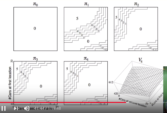 x: number of cars in location B
y: number of cars in location A
================================================================================
Policy improvement in math way
x: number of cars in location B
y: number of cars in location A
================================================================================
Policy improvement in math way
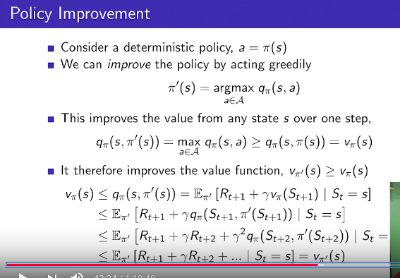 - Goal of proof: if you use policy improvement,
found policy and value function are really optimal?
- Conclusion: Yes.
- Consider deterministic policy, $$$a=\pi(s)$$$
at state s, agent must do action a via policy $$$\pi$$$, not using probability distribution
- Assumption: you can improve the policy $$$\pi$$$ by acting greedily
$$$\pi^{'}(s)=\arg_{a\in A}\max q_{\pi}(s,a)$$$
$$$\pi$$$: previous policy
$$$\pi^{'}$$$: updated policy
-
q(s,a) is action-value function
at states s, via policy $$$\pi$$$, select action a
================================================================================
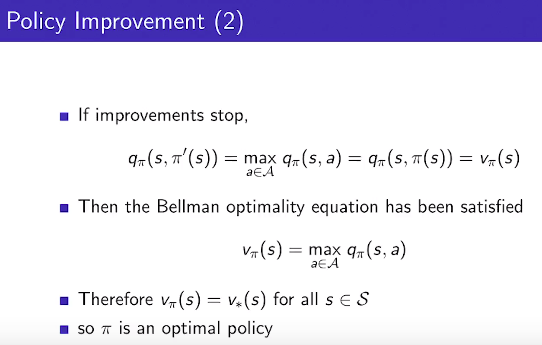
Policy Improvement (2)
- Goal of proof: if you use policy improvement,
found policy and value function are really optimal?
- Conclusion: Yes.
- Consider deterministic policy, $$$a=\pi(s)$$$
at state s, agent must do action a via policy $$$\pi$$$, not using probability distribution
- Assumption: you can improve the policy $$$\pi$$$ by acting greedily
$$$\pi^{'}(s)=\arg_{a\in A}\max q_{\pi}(s,a)$$$
$$$\pi$$$: previous policy
$$$\pi^{'}$$$: updated policy
-
q(s,a) is action-value function
at states s, via policy $$$\pi$$$, select action a
================================================================================
Policy Improvement (2)
 ================================================================================
Modified Policy Iteration
Modified versions of policy iteration
- Should policy evaluation be to converge to $$$v_{\pi}$$$?
- Not allowed early stopping?
- Fixed iteration like 3 evaluation, 3 improves is allowed?
- Conclusion: it makes sense.
================================================================================
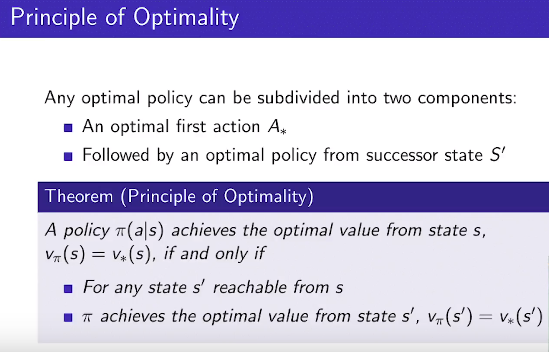
Value iteration
Principle of optimality
================================================================================
Modified Policy Iteration
Modified versions of policy iteration
- Should policy evaluation be to converge to $$$v_{\pi}$$$?
- Not allowed early stopping?
- Fixed iteration like 3 evaluation, 3 improves is allowed?
- Conclusion: it makes sense.
================================================================================
Value iteration
Principle of optimality
 ================================================================================
Deterministic Value Iteation
================================================================================
Deterministic Value Iteation
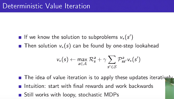 - If you know solution $$$v_{*}(s')$$$ to subproblem $$$s^{'}$$$
- Then, solution $$$v_{*}(s)$$$ of large problem s can be found by using one-step lookahead
- $$$s^{'}$$$: states agent can go from state s
================================================================================
Synchronous Dynamic Programming Algorithm
- If you know solution $$$v_{*}(s')$$$ to subproblem $$$s^{'}$$$
- Then, solution $$$v_{*}(s)$$$ of large problem s can be found by using one-step lookahead
- $$$s^{'}$$$: states agent can go from state s
================================================================================
Synchronous Dynamic Programming Algorithm
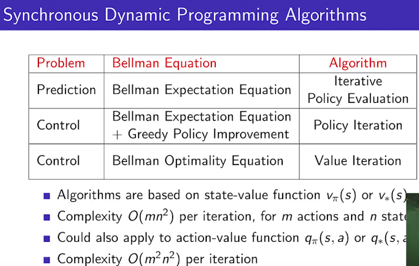 - Dynamic programming algorithm
(synchronous version: update all states at one time)
- You saw "one prediction problems", "two control problems"
- You iteratively use Bellman equation to solve prediction problem
- If algorithms are based on state-value function $$$v_{\pi}(s)$$$ or $$$v_{*}(s)$$$
complexity $$$O(mn^2)$$$ per iteration is large
m: m number of actions
n: n number of states
$$$O(mn^2)$$$: time complexity in big O notation
================================================================================
Asynchronous Dynamic Programming
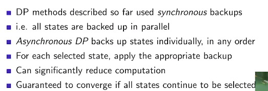
- Dynamic programming algorithm
(synchronous version: update all states at one time)
- You saw "one prediction problems", "two control problems"
- You iteratively use Bellman equation to solve prediction problem
- If algorithms are based on state-value function $$$v_{\pi}(s)$$$ or $$$v_{*}(s)$$$
complexity $$$O(mn^2)$$$ per iteration is large
m: m number of actions
n: n number of states
$$$O(mn^2)$$$: time complexity in big O notation
================================================================================
Asynchronous Dynamic Programming
 ================================================================================
 ================================================================================
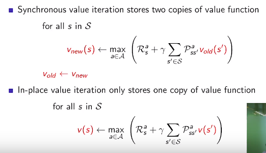
In-Place Dynamic Programming
================================================================================
In-Place Dynamic Programming
 ================================================================================
Prioritised Sweeping
================================================================================
Prioritised Sweeping
 ================================================================================
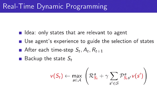
Real-Time Dynamic Programming
================================================================================
Real-Time Dynamic Programming
 ================================================================================
Full-Width Backups
================================================================================
Full-Width Backups
 ================================================================================
Sample Backups
================================================================================
Sample Backups
 ================================================================================