RLCode와 A3C 쉽고 깊게 이해하기
https://www.youtube.com/watch?v=gINks-YCTBs&t=621s
RLCode-A3C.py.html
================================================================================
Table of contents
1. You will see A3C intuitively
1. You will see policy gradient
1. You will see REINFORCE
1. You will see actor-critic
1. You will see A3C
================================================================================
Reinforcement learning has 2 methodologies (value based RL, policy based RL)
A3C uses policy based RL
A3C resolves correlation sample issue by using multiple environments
So, A3C doesn't need to use replay memory
So, A3C became to be able to use policy gradient algorithm
(which is called actor-critic architecture)
A3C shows fast training speed because multiple agents interact with environment at the same time
================================================================================
A3C = asynchronous + actor-critic
A3C is architecture which asynchronously updates actor-critic architecture,
which means A3C can create multiple actor-critic agents and environments
================================================================================
Actor-critic = REINFORCE + online learning
Actor-critic is architecture
which trains REINFORCE algorithm in online way (in other words, real time training)
================================================================================
REINFORCE = Monte Carlo + policy gradient
REINFORCE algorithm is algorithm which updates Monte-Carlo by using policy gradient
Monte-Carlo means, when there are episodes, Monte-Carlo updates itself per every each episode
================================================================================
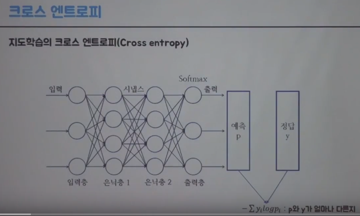
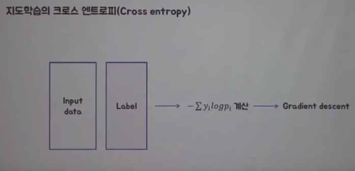
There is cross entropy loss function which is used for supervised learning
Softmax function outputs probabilities in output layer
You assume you have label data y because you suppose you're using supervised learning
Cross entropy loss function in supervised learning can be notated as following:
$$$-\sum y_{i}\log{p_{i}}$$$ which tells you how different between p and y
 ================================================================================
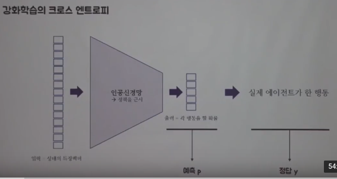
You can use cross entropy loss function for reinforcement learning
Let's say you have policy
And you can approximate that policy into neural network (as like policy network)
That approximated network takes in each state vector as input data
And that approximated network outputs probability of each action which agent can execute
And you can consider the probability as the prediction p
And there should be action which agent actually executed,
and you can consider that action as label y
================================================================================
You can use cross entropy loss function for reinforcement learning
Let's say you have policy
And you can approximate that policy into neural network (as like policy network)
That approximated network takes in each state vector as input data
And that approximated network outputs probability of each action which agent can execute
And you can consider the probability as the prediction p
And there should be action which agent actually executed,
and you can consider that action as label y
 ================================================================================
Then, you can use cross entropy loss function on them (prediction p and action y)
States as input data: $$$s_{0},s_{1},s_{2},...$$$
We input that input data into network which is approximated from policy
Network outputs prediction p representing probability
Actual action which agent executes : $$$a_{0},a_{1},a_{2},...$$$
But it's odd you consider actual action as label data in RL
In other words, action which agent actually executed can't be label (target, goal) of training
So, making prediction same with actually executed action is meaningless
So, in this circumstance, you need kind of direction of update
================================================================================
Then, you can use cross entropy loss function on them (prediction p and action y)
States as input data: $$$s_{0},s_{1},s_{2},...$$$
We input that input data into network which is approximated from policy
Network outputs prediction p representing probability
Actual action which agent executes : $$$a_{0},a_{1},a_{2},...$$$
But it's odd you consider actual action as label data in RL
In other words, action which agent actually executed can't be label (target, goal) of training
So, making prediction same with actually executed action is meaningless
So, in this circumstance, you need kind of direction of update
 ================================================================================
You know q function which represents how actually much good the executed action is
Q function's output q value is summed all future rewards
from specific moment when you selected action
$$$Q_{\pi}(s,a)=E_{\pi}[R_{t+1}+\gamma R_{t+2}+...|S_{t}=s,A_{t}=a]$$$
You can use q function as direction and size of update
And you can say q function in this circumstance as critic
Just like policy is approximated into neural network (policy network, actor network),
q values can be approximated to neural network (q value network, critic network)
In other words, critic uses neural network to know q function
And then you can apply gradient descent on function of
$$$Q(S_{t},A_{t})(-\sum y_{i}\log{p_{i}})$$$
================================================================================
You know q function which represents how actually much good the executed action is
Q function's output q value is summed all future rewards
from specific moment when you selected action
$$$Q_{\pi}(s,a)=E_{\pi}[R_{t+1}+\gamma R_{t+2}+...|S_{t}=s,A_{t}=a]$$$
You can use q function as direction and size of update
And you can say q function in this circumstance as critic
Just like policy is approximated into neural network (policy network, actor network),
q values can be approximated to neural network (q value network, critic network)
In other words, critic uses neural network to know q function
And then you can apply gradient descent on function of
$$$Q(S_{t},A_{t})(-\sum y_{i}\log{p_{i}})$$$
 Actor critic is one agent
Using only one actor critic is slow performance
And it can't resolve correlation sample issue
================================================================================
To resolve above issues,
you can use multiple actor critic agents and environments
Generally, people create 16 agents
Actor critic is one agent
Using only one actor critic is slow performance
And it can't resolve correlation sample issue
================================================================================
To resolve above issues,
you can use multiple actor critic agents and environments
Generally, people create 16 agents
 ================================================================================
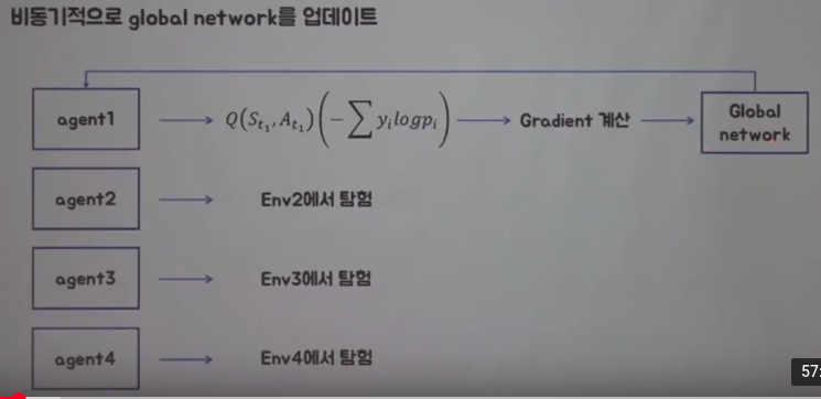
Agent1 can select action from environment1, then you can calculate (q function)*(cross entropy)
And you can say (q function)*(cross entropy) is loss function in reinforcement learning
Then, you apply gradient descent on loss function (q function)*(cross entropy)
And with gradient descent, you can update network
================================================================================
Let's see how update is processed
This is reason A3C has asynchronous term
Agent1 asynchronously updates global network
Other agents keep going tasks
Then, finally global network updates agent1
================================================================================
Agent1 can select action from environment1, then you can calculate (q function)*(cross entropy)
And you can say (q function)*(cross entropy) is loss function in reinforcement learning
Then, you apply gradient descent on loss function (q function)*(cross entropy)
And with gradient descent, you can update network
================================================================================
Let's see how update is processed
This is reason A3C has asynchronous term
Agent1 asynchronously updates global network
Other agents keep going tasks
Then, finally global network updates agent1
 ================================================================================
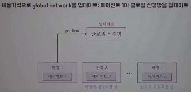
Agent1 updates global network
You can see multiple agents and multiple environments
================================================================================
Agent1 updates global network
You can see multiple agents and multiple environments
 ================================================================================
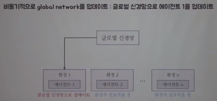
Global network updates agent1
================================================================================
Global network updates agent1
 ================================================================================
Goal of reinforcement learning is to increase probability of occuring action which gives most reward
That is, policy means rules which agent uses when selecting action at each state
That is, you should update "current policy" based on "reward" obtained from environment
It means you need
1."criterion" which is used when updating policy
2."way of updating" policy, based on that criterion
With knowledge of them, you can know how to process policy gradient
"Criterion for updating policy" will be "target function"
which is not one kind and what agent should learn
"Way for updating policy" will be gradient ascent applied on target function to update policy
Policy
-> target function $$$J(\theta)$$$ of policy
-> Apply gradient ascent on $$$J(\theta)$$$ to maximize $$$J(\theta)$$$
-> Then you will obtain optimal policy
================================================================================
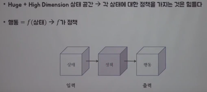
First, you should consider to approximate policy
If state of question which agent wants to learn is huge and high dimension,
it's almost impossible for agent to have all policies on each state
So, you need to consider states as input value to function f,
Then, you approximate policy into function f.
It means output from function f is action
================================================================================
Goal of reinforcement learning is to increase probability of occuring action which gives most reward
That is, policy means rules which agent uses when selecting action at each state
That is, you should update "current policy" based on "reward" obtained from environment
It means you need
1."criterion" which is used when updating policy
2."way of updating" policy, based on that criterion
With knowledge of them, you can know how to process policy gradient
"Criterion for updating policy" will be "target function"
which is not one kind and what agent should learn
"Way for updating policy" will be gradient ascent applied on target function to update policy
Policy
-> target function $$$J(\theta)$$$ of policy
-> Apply gradient ascent on $$$J(\theta)$$$ to maximize $$$J(\theta)$$$
-> Then you will obtain optimal policy
================================================================================
First, you should consider to approximate policy
If state of question which agent wants to learn is huge and high dimension,
it's almost impossible for agent to have all policies on each state
So, you need to consider states as input value to function f,
Then, you approximate policy into function f.
It means output from function f is action
 ================================================================================
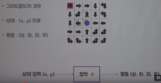
Each arrow is each policy at each state (each mini square)
So you will use x y coordinates to represent state as input data
You will use policy in the form of approximated policy function $$$\pi$$$
Then, policy function outputs the action out of up,down,right,left
================================================================================
Each arrow is each policy at each state (each mini square)
So you will use x y coordinates to represent state as input data
You will use policy in the form of approximated policy function $$$\pi$$$
Then, policy function outputs the action out of up,down,right,left
 ================================================================================
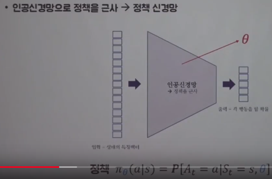
There can be various ways to approximate policy
You will approximate policy into policy function by using deep learning methodology
In other words, it means policy function will be neural network
Now, what you should do is to define input and output in neural network
================================================================================
$$$\pi(a|s)=P[A_{t}=a|S_{t}=s]$$$:
- policy $$$\pi$$$ means conditional probability of a occurring, at given state s
- $$$\pi(a|s)$$$: raw notation of policy
$$$\pi_\theta(a|s)=P[A_{t}=a|S_{t}=s,\theta]$$$:
- You can write above notation by adding $$$\theta$$$ term
because you appoximate policy $$$\pi$$$ by neural network $$$\theta$$$
- $$$\pi_\theta(a|s)$$$: approximated policy by neural network $$$\theta$$$
================================================================================
Since you're using neural network, you should intialize neural network
Then you will inevitably obtain meaningless initialization value at very initial moment
Goal you will achieve is update that neural network (initialization value)
================================================================================
There can be various ways to approximate policy
You will approximate policy into policy function by using deep learning methodology
In other words, it means policy function will be neural network
Now, what you should do is to define input and output in neural network
================================================================================
$$$\pi(a|s)=P[A_{t}=a|S_{t}=s]$$$:
- policy $$$\pi$$$ means conditional probability of a occurring, at given state s
- $$$\pi(a|s)$$$: raw notation of policy
$$$\pi_\theta(a|s)=P[A_{t}=a|S_{t}=s,\theta]$$$:
- You can write above notation by adding $$$\theta$$$ term
because you appoximate policy $$$\pi$$$ by neural network $$$\theta$$$
- $$$\pi_\theta(a|s)$$$: approximated policy by neural network $$$\theta$$$
================================================================================
Since you're using neural network, you should intialize neural network
Then you will inevitably obtain meaningless initialization value at very initial moment
Goal you will achieve is update that neural network (initialization value)
 ================================================================================
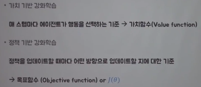
In RL, there are 2 streams (value based reinforcement learnig, policy based reinforcement learnig)
Value based reinforcement learnig:
Criterion which agent uses to select action at every step is value function (i.e. q function)
Policy based reinforcement learnig
Criterion which agent uses to select action at every update is target function $$$J(\theta)$$$
$$$\theta$$$ is neural network which approximated policy
================================================================================
In RL, there are 2 streams (value based reinforcement learnig, policy based reinforcement learnig)
Value based reinforcement learnig:
Criterion which agent uses to select action at every step is value function (i.e. q function)
Policy based reinforcement learnig
Criterion which agent uses to select action at every update is target function $$$J(\theta)$$$
$$$\theta$$$ is neural network which approximated policy
 ================================================================================
Let's think about pathway
which agent will walk along based on policy $$$\pi_{\theta}$$$
And you will call that pathway as trajectory $$$\tau$$$,
which represents trace of interaction between agent and environment
$$$s_{0}$$$: initial state
$$$a_{0}$$$: initail chosen action basend on policy
$$$r_{1}$$$: reward
Entire trajectory $$$\tau=s_{0},a_{0},r_{1},s_{1},a_{1},r_{2},...,s_{T}$$$
Since network outputs action, trajectory can differ whenever it goes
So, you can use technique of expectation to resolve above trouble
$$$J(\theta)=E[\sum\limits_{t=0}^{T-1}r_{t+1}|\pi_{\theta}] $$$
$$$J(\theta)=E[r_{1}+r_{2}+r_{3}+...+r_{T}|\pi_{\theta}]$$$
$$$J(\theta)$$$ is target function which agent should increase
Agent has target function $$$J(\theta)$$$ which agent should increase
================================================================================
You will update neural network $$$\theta$$$,
by using gradient ascent on target function $$$J(\theta)$$$
$$$\theta'=\theta+\alpha \nabla_{\theta}J(\theta)$$$
$$$\theta'$$$ : new updated policy
$$$\theta$$$ : current policy
You first find target function J(\theta) in repect to trajectory which agent experienced
Then, you perform gradient on $$$J(\theta)$$$
$$$\nabla_{\theta}J(\theta)$$$ : policy gradient
In other words, policy gradient is differentiation of target function J(\theta)
in respect to network $$$\theta$$$
================================================================================
Basic algorithm which performs policy gradient is REINFORCE
REINFORCE can be notated as following
$$$\nabla_{\theta}J(\theta)\sim \sum\limits_{t=0}^{T-1} \nabla_{\theta}\log{\pi_{\theta}}(a_{t}|s_{t})G_{t}$$$
Again, target function $$$J(\theta)$$$ for policy gradient can be also notated as following
$$$J(\theta)=E[\sum\limits_{t=0}^{T-1}r_{t+1}|\pi_{\theta}]$$$
When approximated policy $$$\pi_{\theta}$$$ is given,
expection value of $$$r_{1}+...r_{T}$$$ is target function $$$J(\theta)$$$
T: terminal moment
Agent should maximize above target function by using gradient ascent
Expectation value = sum of (probability of occurring x)*(value at x) in respect to x
For example, expectation value from dice
$$$E[f(x)]=\sum\limits_{x}p(x)f(x)$$$
When trajectory $$$\tau = s_{0},a_{0},r_{1},s_{1},a_{1},r_{2},...,s_{T}$$$
target function $$$J(\theta)$$$ can be notated as following
$$$J(\theta)=E[\sum\limits_{t=1}^{T-1}r_{t+1}|\pi_{\theta}]$$$
$$$J(\theta)=E_{\tau}[r_{1}|\pi_{\theta}] + E_{\tau}[r_{2}|\pi_{\theta}] + E_{\tau}[r_{3}|\pi_{\theta}] + ...$$$
$$$E_{\tau}[r_{1}|\pi_{\theta}]$$$ : expectation value in respect to $$$r_{1}$$$ at trajectory $$$\tau$$$
$$$J(\theta)=\sum\limits_{t=0}^{T-1}P(s_{t},a_{t}|\tau)R(s_{t},a_{t})$$$
$$$P(s_{t},a_{t}|\tau)$$$ : probability of occuring $$$(s_{t},a_{t})$$$
$$$R(s_{t},a_{t})$$$ : value at $$$(s_{t},a_{t})$$$
$$$J(\theta)=\sum\limits_{t=0}^{T-1}P(s_{t},a_{t}|\tau)r_{t+1}$$$
Perform $$$\nabla_{\theta}$$$ (differentiation) on both side
$$$\nabla_{\theta}J(\theta)=\nabla_{\theta} E[\sum\limits_{t=1}^{T-1}r_{t+1}|\pi_{\theta}]$$$
$$$\nabla_{\theta}J(\theta)=\nabla_{\theta} \sum\limits_{t=0}^{T-1} P(s_{t},a_{t}|\tau)r_{t+1}$$$
$$$\nabla_{\theta}J(\theta)=\sum\limits_{t=0}^{T-1} \nabla_{\theta} P(s_{t},a_{t}|\tau)r_{t+1}$$$
We will inspect this step more detail
$$$\nabla_{\theta}J(\theta)=\sum\limits_{t=0}^{T-1} P(s_{t},a_{t}|\tau) \nabla_{\theta} \log{P(s_{t},a_{t}|\tau)r_{t+1}} $$$
Detailed step:
$$$\nabla_{\theta}J(\theta)=\sum\limits_{t=0}^{T-1} \nabla_{\theta} P(s_{t},a_{t}|\tau)r_{t+1}$$$
According to characteristic of log differentiation
$$$\frac{d}{dx}\log{x}=\frac{1}{x}$$$
$$$\frac{d}{dx}\log{f(x)}=\frac{\frac{d}{dx}f(x)}{f(x)}$$$
$$$\nabla_{\theta}J(\theta) = \sum\limits_{t=0}^{T-1} P(s_{t},a_{t}|\tau) \frac{\nabla_{\theta} P(s_{t},a_{t}|\tau)}{P(s_{t},a_{t}|\tau)} r_{t+1}$$$
Finally,
$$$\nabla_{\theta}J(\theta) = \sum\limits_{t=0}^{T-1} P(s_{t},a_{t}|\tau) \nabla_{\theta} \log{P(s_{t},a_{t}|\tau)r_{t+1}}$$$
You convert above formular into expectation value notation
$$$\nabla_{\theta}J(\theta) = E_{\tau}[\sum\limits_{t=0}^{T-1} \nabla_{\theta} \log{P(s_{t},a_{t}|\tau)r_{t+1}}]$$$
When it comes to reinforcement learning,
you can't calculate E[],
so you do sampling,
which means you do one try and calculate and the update,
you do second try and calculate and the update,...
$$$\rightarrow \sum\limits_{t=0}^{T-1}\nabla_{\theta}\log{P(s_{t},a_{t}|\tau)r_{t+1}}$$$
You should find $$$\log{P(s_{t},a_{t}|\tau)}$$$ to go further
$$$P(s_{t},a_{t}|\tau)=P(s_{0},a_{0},r_{1},s_{1},a_{1},r_{2},...,s_{t},a_{t}|\theta])$$$
You will see traces of interaction between agent and environment from following notation
$$$P(s_{t},a_{t}|\tau)=P(s_{0})\pi_{\theta}(a_{0}|s_{0}) P(s_{1}|s_{0},a_{0})\pi_{\theta}(a_{1}|s_{1}) P(s_{2}|s_{1},a_{1})...$$$
P is environment
$$$\pi$$$ is agent
Agent can't know P
We can try to perform log on both side
$$$\log{P(s_{t},a_{t}|\tau)}=\log{} P(s_{0})\pi_{\theta}(a_{0}|s_{0}) P(s_{1}|s_{0},a_{0})\pi_{\theta}(a_{1}|s_{1}) ... P(s_{t}|s_{t-1},a_{t-1})\pi_{\theta}(a_{t}|s_{t})$$$
We can use following rule,
$$$\log{AB}=\log{A}+\log{B}$$$
$$$\log{P(s_{t},a_{t}|\tau)}=\log{P(s_{0})} + \log{\pi_{\theta}(a_{0}|s_{0})} + \log{P(s_{1}|s_{0},a_{0})} + \log{\pi_{\theta}(a_{1}|s_{1})} + ... + \log{P(s_{t}|s_{t-1},a_{t-1})} + \log{\pi_{\theta}(a_{t}|s_{t})}$$$
...
To do writing formulars
================================================================================
REINFORCE
1. You run one episode based on current policy
1. You record trajectory which is obtained from each episode
1. When episode ends, you calculate $$$G_{t}$$$
If trajectory is 100 steps, it means you obtain 100 returns
1. You calculate policy gradient, then update policy
1. You iterate above 1-4 steps
Since you update policy per episode,
you call this way as Monte Carlo policy gradient, or simply REINFORCE
Updating policy per "episode" can't be called "online"
================================================================================
Issue of REINFORCE
1. It creates high variance
because as episode becomes longer, you can run into various trajectory
1. You only can update policy per episode (you can't use online learning)
Resolving ways:
1. You can upgrade from Monte Carlo to TD (Temporal Difference)
Temporal Difference means you update policy more often than Monte Carlo,
Monte Carlo means you update policy when episode is finished
1. You can upgrade from Monte Carlo to Actor-Critic
Actor-Critic means you update policy per each step
================================================================================
Simply, actor-critic means you use 2 networks
One (actor network) will be used as policy network
One (critic network) will be used as q function network
Critic (q function) can be considered as critic person
who criticizes agent's action with saying that action is either good or bad
Then, you can update policy per every step
================================================================================
You won't use q function as it is.
For example, suppose moving to right is +2 reward which means good action.
Suposse moving to left is +1 reward which means bad action.
But if we consider reward of moving to right as +1, reward of moving to left as -1,
task of update and training will be easier
Therefore, to achieve above technique,
you will use advantage function instead of q function.
Advantage function can be generated by (q function) - (baseline (value function) which means average reward)
By substacting them, it reduces variance
================================================================================
Q function means value from at specific state, by specific action
Value function is baseline,
value function is value from at specific state, by general action
================================================================================
Approximating both Q and V is inefficient.
So, you will use following formular
$$$Q(s_{t},a_{t})=E[r_{t+1}+\gamma V(s_{t+1})|s_{t},a_{t}]$$$
Then,
$$$\nabla_{\theta}J(\theta)\sim \nabla_{\theta}\log{\pi_{\theta}(a_{t}|s_{t})}(r_{t+1}+\gamma V_{v}(s_{t+1})-V_{v}(s_{t}))$$$
You can consider $$$r_{t+1}+\gamma V_{v}(s_{t+1})$$$ as q function
You can consider $$$V_{v}(s_{t})$$$ as baseline
================================================================================
Actor approximates policy to $$$\theta$$$
You update actor network by using following actor's loss function
$$$\nabla_{\theta}\log{\pi_{\theta}}(a_{t}|s_{t})(r_{t+1}+\gamma V_{v}(s_{t+1}-V_{v}(s_{t}))$$$
Critic approximates value function to v
You update critic network by using following MSE loss function
$$$(r_{t+1}+\gamma V_{v}(s_{t+1})-V_{v}(s_{t}))^{2}$$$
================================================================================
Actor network (policy network) outputs probability of action
Critic network (value network) outputs value
You can update actor network (policy network) by using actor network's loss function (cross entropy)*(TD error)
$$$-\nabla_{\theta}\log{\pi_{\theta}}(a_{t}|s_{t})(r_{t+1}+\gamma V_{v}(s_{t+1}-V_{v}(s_{t}))$$$
Actor network can create cross entropy part $$$\nabla_{\theta}\log{\pi_{\theta}}(a_{t}|s_{t})$$$
Then actor network can bring TD error part $$$(r_{t+1}+\gamma V_{v}(s_{t+1}-V_{v}(s_{t}))$$$ from critic network
You can update critic network (value network) by using TD error
After update, you proceed one step more, then you can update again,
which means you update per step unlike REINFORCE,
which should reach end of episode to update network
Actor network (value network) calculates value,
representing how much good action at each step is
================================================================================
Let's think about pathway
which agent will walk along based on policy $$$\pi_{\theta}$$$
And you will call that pathway as trajectory $$$\tau$$$,
which represents trace of interaction between agent and environment
$$$s_{0}$$$: initial state
$$$a_{0}$$$: initail chosen action basend on policy
$$$r_{1}$$$: reward
Entire trajectory $$$\tau=s_{0},a_{0},r_{1},s_{1},a_{1},r_{2},...,s_{T}$$$
Since network outputs action, trajectory can differ whenever it goes
So, you can use technique of expectation to resolve above trouble
$$$J(\theta)=E[\sum\limits_{t=0}^{T-1}r_{t+1}|\pi_{\theta}] $$$
$$$J(\theta)=E[r_{1}+r_{2}+r_{3}+...+r_{T}|\pi_{\theta}]$$$
$$$J(\theta)$$$ is target function which agent should increase
Agent has target function $$$J(\theta)$$$ which agent should increase
================================================================================
You will update neural network $$$\theta$$$,
by using gradient ascent on target function $$$J(\theta)$$$
$$$\theta'=\theta+\alpha \nabla_{\theta}J(\theta)$$$
$$$\theta'$$$ : new updated policy
$$$\theta$$$ : current policy
You first find target function J(\theta) in repect to trajectory which agent experienced
Then, you perform gradient on $$$J(\theta)$$$
$$$\nabla_{\theta}J(\theta)$$$ : policy gradient
In other words, policy gradient is differentiation of target function J(\theta)
in respect to network $$$\theta$$$
================================================================================
Basic algorithm which performs policy gradient is REINFORCE
REINFORCE can be notated as following
$$$\nabla_{\theta}J(\theta)\sim \sum\limits_{t=0}^{T-1} \nabla_{\theta}\log{\pi_{\theta}}(a_{t}|s_{t})G_{t}$$$
Again, target function $$$J(\theta)$$$ for policy gradient can be also notated as following
$$$J(\theta)=E[\sum\limits_{t=0}^{T-1}r_{t+1}|\pi_{\theta}]$$$
When approximated policy $$$\pi_{\theta}$$$ is given,
expection value of $$$r_{1}+...r_{T}$$$ is target function $$$J(\theta)$$$
T: terminal moment
Agent should maximize above target function by using gradient ascent
Expectation value = sum of (probability of occurring x)*(value at x) in respect to x
For example, expectation value from dice
$$$E[f(x)]=\sum\limits_{x}p(x)f(x)$$$
When trajectory $$$\tau = s_{0},a_{0},r_{1},s_{1},a_{1},r_{2},...,s_{T}$$$
target function $$$J(\theta)$$$ can be notated as following
$$$J(\theta)=E[\sum\limits_{t=1}^{T-1}r_{t+1}|\pi_{\theta}]$$$
$$$J(\theta)=E_{\tau}[r_{1}|\pi_{\theta}] + E_{\tau}[r_{2}|\pi_{\theta}] + E_{\tau}[r_{3}|\pi_{\theta}] + ...$$$
$$$E_{\tau}[r_{1}|\pi_{\theta}]$$$ : expectation value in respect to $$$r_{1}$$$ at trajectory $$$\tau$$$
$$$J(\theta)=\sum\limits_{t=0}^{T-1}P(s_{t},a_{t}|\tau)R(s_{t},a_{t})$$$
$$$P(s_{t},a_{t}|\tau)$$$ : probability of occuring $$$(s_{t},a_{t})$$$
$$$R(s_{t},a_{t})$$$ : value at $$$(s_{t},a_{t})$$$
$$$J(\theta)=\sum\limits_{t=0}^{T-1}P(s_{t},a_{t}|\tau)r_{t+1}$$$
Perform $$$\nabla_{\theta}$$$ (differentiation) on both side
$$$\nabla_{\theta}J(\theta)=\nabla_{\theta} E[\sum\limits_{t=1}^{T-1}r_{t+1}|\pi_{\theta}]$$$
$$$\nabla_{\theta}J(\theta)=\nabla_{\theta} \sum\limits_{t=0}^{T-1} P(s_{t},a_{t}|\tau)r_{t+1}$$$
$$$\nabla_{\theta}J(\theta)=\sum\limits_{t=0}^{T-1} \nabla_{\theta} P(s_{t},a_{t}|\tau)r_{t+1}$$$
We will inspect this step more detail
$$$\nabla_{\theta}J(\theta)=\sum\limits_{t=0}^{T-1} P(s_{t},a_{t}|\tau) \nabla_{\theta} \log{P(s_{t},a_{t}|\tau)r_{t+1}} $$$
Detailed step:
$$$\nabla_{\theta}J(\theta)=\sum\limits_{t=0}^{T-1} \nabla_{\theta} P(s_{t},a_{t}|\tau)r_{t+1}$$$
According to characteristic of log differentiation
$$$\frac{d}{dx}\log{x}=\frac{1}{x}$$$
$$$\frac{d}{dx}\log{f(x)}=\frac{\frac{d}{dx}f(x)}{f(x)}$$$
$$$\nabla_{\theta}J(\theta) = \sum\limits_{t=0}^{T-1} P(s_{t},a_{t}|\tau) \frac{\nabla_{\theta} P(s_{t},a_{t}|\tau)}{P(s_{t},a_{t}|\tau)} r_{t+1}$$$
Finally,
$$$\nabla_{\theta}J(\theta) = \sum\limits_{t=0}^{T-1} P(s_{t},a_{t}|\tau) \nabla_{\theta} \log{P(s_{t},a_{t}|\tau)r_{t+1}}$$$
You convert above formular into expectation value notation
$$$\nabla_{\theta}J(\theta) = E_{\tau}[\sum\limits_{t=0}^{T-1} \nabla_{\theta} \log{P(s_{t},a_{t}|\tau)r_{t+1}}]$$$
When it comes to reinforcement learning,
you can't calculate E[],
so you do sampling,
which means you do one try and calculate and the update,
you do second try and calculate and the update,...
$$$\rightarrow \sum\limits_{t=0}^{T-1}\nabla_{\theta}\log{P(s_{t},a_{t}|\tau)r_{t+1}}$$$
You should find $$$\log{P(s_{t},a_{t}|\tau)}$$$ to go further
$$$P(s_{t},a_{t}|\tau)=P(s_{0},a_{0},r_{1},s_{1},a_{1},r_{2},...,s_{t},a_{t}|\theta])$$$
You will see traces of interaction between agent and environment from following notation
$$$P(s_{t},a_{t}|\tau)=P(s_{0})\pi_{\theta}(a_{0}|s_{0}) P(s_{1}|s_{0},a_{0})\pi_{\theta}(a_{1}|s_{1}) P(s_{2}|s_{1},a_{1})...$$$
P is environment
$$$\pi$$$ is agent
Agent can't know P
We can try to perform log on both side
$$$\log{P(s_{t},a_{t}|\tau)}=\log{} P(s_{0})\pi_{\theta}(a_{0}|s_{0}) P(s_{1}|s_{0},a_{0})\pi_{\theta}(a_{1}|s_{1}) ... P(s_{t}|s_{t-1},a_{t-1})\pi_{\theta}(a_{t}|s_{t})$$$
We can use following rule,
$$$\log{AB}=\log{A}+\log{B}$$$
$$$\log{P(s_{t},a_{t}|\tau)}=\log{P(s_{0})} + \log{\pi_{\theta}(a_{0}|s_{0})} + \log{P(s_{1}|s_{0},a_{0})} + \log{\pi_{\theta}(a_{1}|s_{1})} + ... + \log{P(s_{t}|s_{t-1},a_{t-1})} + \log{\pi_{\theta}(a_{t}|s_{t})}$$$
...
To do writing formulars
================================================================================
REINFORCE
1. You run one episode based on current policy
1. You record trajectory which is obtained from each episode
1. When episode ends, you calculate $$$G_{t}$$$
If trajectory is 100 steps, it means you obtain 100 returns
1. You calculate policy gradient, then update policy
1. You iterate above 1-4 steps
Since you update policy per episode,
you call this way as Monte Carlo policy gradient, or simply REINFORCE
Updating policy per "episode" can't be called "online"
================================================================================
Issue of REINFORCE
1. It creates high variance
because as episode becomes longer, you can run into various trajectory
1. You only can update policy per episode (you can't use online learning)
Resolving ways:
1. You can upgrade from Monte Carlo to TD (Temporal Difference)
Temporal Difference means you update policy more often than Monte Carlo,
Monte Carlo means you update policy when episode is finished
1. You can upgrade from Monte Carlo to Actor-Critic
Actor-Critic means you update policy per each step
================================================================================
Simply, actor-critic means you use 2 networks
One (actor network) will be used as policy network
One (critic network) will be used as q function network
Critic (q function) can be considered as critic person
who criticizes agent's action with saying that action is either good or bad
Then, you can update policy per every step
================================================================================
You won't use q function as it is.
For example, suppose moving to right is +2 reward which means good action.
Suposse moving to left is +1 reward which means bad action.
But if we consider reward of moving to right as +1, reward of moving to left as -1,
task of update and training will be easier
Therefore, to achieve above technique,
you will use advantage function instead of q function.
Advantage function can be generated by (q function) - (baseline (value function) which means average reward)
By substacting them, it reduces variance
================================================================================
Q function means value from at specific state, by specific action
Value function is baseline,
value function is value from at specific state, by general action
================================================================================
Approximating both Q and V is inefficient.
So, you will use following formular
$$$Q(s_{t},a_{t})=E[r_{t+1}+\gamma V(s_{t+1})|s_{t},a_{t}]$$$
Then,
$$$\nabla_{\theta}J(\theta)\sim \nabla_{\theta}\log{\pi_{\theta}(a_{t}|s_{t})}(r_{t+1}+\gamma V_{v}(s_{t+1})-V_{v}(s_{t}))$$$
You can consider $$$r_{t+1}+\gamma V_{v}(s_{t+1})$$$ as q function
You can consider $$$V_{v}(s_{t})$$$ as baseline
================================================================================
Actor approximates policy to $$$\theta$$$
You update actor network by using following actor's loss function
$$$\nabla_{\theta}\log{\pi_{\theta}}(a_{t}|s_{t})(r_{t+1}+\gamma V_{v}(s_{t+1}-V_{v}(s_{t}))$$$
Critic approximates value function to v
You update critic network by using following MSE loss function
$$$(r_{t+1}+\gamma V_{v}(s_{t+1})-V_{v}(s_{t}))^{2}$$$
================================================================================
Actor network (policy network) outputs probability of action
Critic network (value network) outputs value
You can update actor network (policy network) by using actor network's loss function (cross entropy)*(TD error)
$$$-\nabla_{\theta}\log{\pi_{\theta}}(a_{t}|s_{t})(r_{t+1}+\gamma V_{v}(s_{t+1}-V_{v}(s_{t}))$$$
Actor network can create cross entropy part $$$\nabla_{\theta}\log{\pi_{\theta}}(a_{t}|s_{t})$$$
Then actor network can bring TD error part $$$(r_{t+1}+\gamma V_{v}(s_{t+1}-V_{v}(s_{t}))$$$ from critic network
You can update critic network (value network) by using TD error
After update, you proceed one step more, then you can update again,
which means you update per step unlike REINFORCE,
which should reach end of episode to update network
Actor network (value network) calculates value,
representing how much good action at each step is
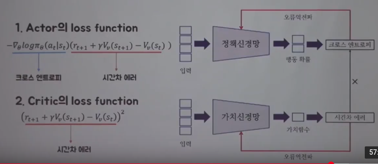 ================================================================================
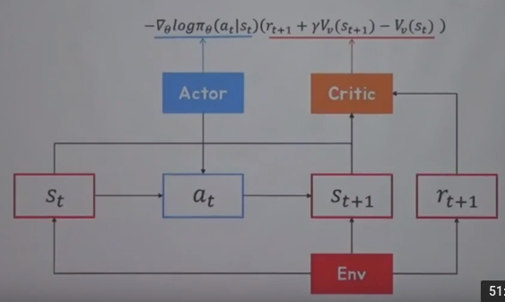
Illustration between actor and critic
At state $$$s_{t}$$$, actor network selects action $$$a_{t}$$$,
then, environment tells next state $$$s_{t+1}$$$ and instant reward $$$r_{t+1}$$$
And actor network creates cross entropy part $$$\nabla_{\theta}\log{\pi_{\theta}}(a_{t}|s_{t})$$$
Critic network takes in $$$s_{t+1}$$$ and $$$r_{t+1}$$$ to calculate TD error $$$(r_{t+1}+\gamma V_{v}(s_{t+1}-V_{v}(s_{t}))$$$
Then, critic network updates critic network by above TD error
Then actor multiplies cross entropy by TD error generated by critic network
$$$\nabla_{\theta}\log{\pi_{\theta}}(a_{t}|s_{t})(r_{t+1}+\gamma V_{v}(s_{t+1}-V_{v}(s_{t}))$$$
With above formular, actor network updates actor network
================================================================================
Illustration between actor and critic
At state $$$s_{t}$$$, actor network selects action $$$a_{t}$$$,
then, environment tells next state $$$s_{t+1}$$$ and instant reward $$$r_{t+1}$$$
And actor network creates cross entropy part $$$\nabla_{\theta}\log{\pi_{\theta}}(a_{t}|s_{t})$$$
Critic network takes in $$$s_{t+1}$$$ and $$$r_{t+1}$$$ to calculate TD error $$$(r_{t+1}+\gamma V_{v}(s_{t+1}-V_{v}(s_{t}))$$$
Then, critic network updates critic network by above TD error
Then actor multiplies cross entropy by TD error generated by critic network
$$$\nabla_{\theta}\log{\pi_{\theta}}(a_{t}|s_{t})(r_{t+1}+\gamma V_{v}(s_{t+1}-V_{v}(s_{t}))$$$
With above formular, actor network updates actor network
 ================================================================================
A3C:
In especially process of update, actor critic processes update like one step, one update,
However, a3c goes 5 steps or 10 steps or any multi steps then it asynchronously updates
loss function after 1 step:
$$$\nabla_{\theta}\log{\pi_{\theta}(a_{t}|s_{t})}(r_{t+1}+\gamma V_{v}(s_{t+1})-V_{v}(s_{t}))$$$
loss function after 2 step:
$$$\nabla_{\theta}\log{\pi_{\theta}(a_{t}|s_{t})}(r_{t+1}+\gamma r_{t+2}+\gamma^{2} V_{v}(s_{t+2})-V_{v}(s_{t}))$$$
...
loss function after 20 step:
$$$\nabla_{\theta}\log{\pi_{\theta}(a_{t}|s_{t})}(r_{t+1}+\gamma r_{t+2}+...+\gamma^{19}V_{v}(s_{t+20})-V_{v}(s_{t}))$$$
If you go 20 steps, after 20 steps, you obtain one loss function like above formulars
Until 19 steps, you add actual reward you obtain, at 20 step, you use value function,
which means you create multi steps
Since you put more step information into loss function, precision will increase, with decreasing bias
But you actually will use all 20 loss functions by summing them all
$$$\text{Final loss function L}=\nabla_{\theta}\log{\pi_{\theta}(a_{t}|s_{t})}(r_{t+1}+\gamma r_{t+2}+...+\gamma^{19}V_{v}(s_{t+20})-V_{v}(s_{t})) + \nabla_{\theta}\log{\pi_{\theta}(a_{t+1}|s_{t+1})}(r_{t+2}+\gamma r_{t+3}+...+\gamma^{18}V_{v}(s_{t+20})-V_{v}(s_{t+1})) + \nabla_{\theta}\log{\pi_{\theta}(a_{t+2}|s_{t+2})}(r_{t+3}+\gamma r_{t+4}+...+\gamma^{17}V_{v}(s_{t+20})-V_{v}(s_{t+2})) + ... + \nabla_{\theta}\log{\pi_{\theta}(a_{t+19}|s_{t+19})}(r_{t+19}+\gamma V_{v}(s_{t+20}) - V_{v}(s_{t+19}))$$$
================================================================================
Actor-critic's loss function:
$$$-\nabla\log{\pi_{\theta}(a_{t}|s_{t})}(r_{t+1}+\gamma V_{v}(s_{t+1}-V_{v}(s_{t})))$$$
A3C's loss function
$$$-\nabla\log{\pi_{\theta}(a_{t+19}|s_{t+19})}(r_{t+1}+...+\gamma^{19} V_{v}(s_{t+20})-V_{v}(s_{t}))...+\sum\limits_{t=0}^{19}\sum\limits_{i}p_{i}\log{p_{i}}$$$
$$$-\nabla\log{\pi_{\theta}(a_{t+19}|s_{t+19})}(r_{t+1}+...+\gamma^{19} V_{v}(s_{t+20})-V_{v}(s_{t}))...$$$ is 20 cross entropies:
which means exploitation, which means you update network with knowledge which you have
$$$\sum\limits_{t=0}^{19}\sum\limits_{i}p_{i}\log{p_{i}}$$$: Entropy:
which means exploration which means you let agent to do more exploration
================================================================================
A3C:
In especially process of update, actor critic processes update like one step, one update,
However, a3c goes 5 steps or 10 steps or any multi steps then it asynchronously updates
loss function after 1 step:
$$$\nabla_{\theta}\log{\pi_{\theta}(a_{t}|s_{t})}(r_{t+1}+\gamma V_{v}(s_{t+1})-V_{v}(s_{t}))$$$
loss function after 2 step:
$$$\nabla_{\theta}\log{\pi_{\theta}(a_{t}|s_{t})}(r_{t+1}+\gamma r_{t+2}+\gamma^{2} V_{v}(s_{t+2})-V_{v}(s_{t}))$$$
...
loss function after 20 step:
$$$\nabla_{\theta}\log{\pi_{\theta}(a_{t}|s_{t})}(r_{t+1}+\gamma r_{t+2}+...+\gamma^{19}V_{v}(s_{t+20})-V_{v}(s_{t}))$$$
If you go 20 steps, after 20 steps, you obtain one loss function like above formulars
Until 19 steps, you add actual reward you obtain, at 20 step, you use value function,
which means you create multi steps
Since you put more step information into loss function, precision will increase, with decreasing bias
But you actually will use all 20 loss functions by summing them all
$$$\text{Final loss function L}=\nabla_{\theta}\log{\pi_{\theta}(a_{t}|s_{t})}(r_{t+1}+\gamma r_{t+2}+...+\gamma^{19}V_{v}(s_{t+20})-V_{v}(s_{t})) + \nabla_{\theta}\log{\pi_{\theta}(a_{t+1}|s_{t+1})}(r_{t+2}+\gamma r_{t+3}+...+\gamma^{18}V_{v}(s_{t+20})-V_{v}(s_{t+1})) + \nabla_{\theta}\log{\pi_{\theta}(a_{t+2}|s_{t+2})}(r_{t+3}+\gamma r_{t+4}+...+\gamma^{17}V_{v}(s_{t+20})-V_{v}(s_{t+2})) + ... + \nabla_{\theta}\log{\pi_{\theta}(a_{t+19}|s_{t+19})}(r_{t+19}+\gamma V_{v}(s_{t+20}) - V_{v}(s_{t+19}))$$$
================================================================================
Actor-critic's loss function:
$$$-\nabla\log{\pi_{\theta}(a_{t}|s_{t})}(r_{t+1}+\gamma V_{v}(s_{t+1}-V_{v}(s_{t})))$$$
A3C's loss function
$$$-\nabla\log{\pi_{\theta}(a_{t+19}|s_{t+19})}(r_{t+1}+...+\gamma^{19} V_{v}(s_{t+20})-V_{v}(s_{t}))...+\sum\limits_{t=0}^{19}\sum\limits_{i}p_{i}\log{p_{i}}$$$
$$$-\nabla\log{\pi_{\theta}(a_{t+19}|s_{t+19})}(r_{t+1}+...+\gamma^{19} V_{v}(s_{t+20})-V_{v}(s_{t}))...$$$ is 20 cross entropies:
which means exploitation, which means you update network with knowledge which you have
$$$\sum\limits_{t=0}^{19}\sum\limits_{i}p_{i}\log{p_{i}}$$$: Entropy:
which means exploration which means you let agent to do more exploration
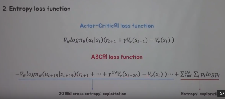 ================================================================================
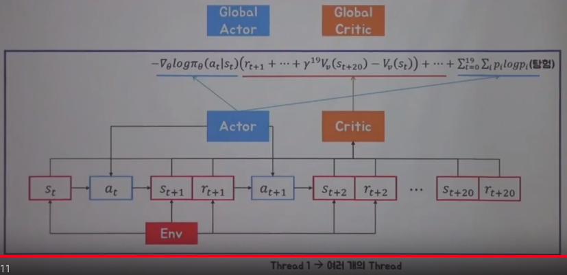
Illustration of overview step on A3C
You start from $$$s_{t}$$$, and you will go 20 steps
Critic gets red boxes values to create red underline term
Actor creates 2 terms (one is exploitation term, one is exploration term by other agents)
You update global actor network and global critic network by combined loss function
Above process is running on 1 thread, you can create multiple threads
================================================================================
Illustration of overview step on A3C
You start from $$$s_{t}$$$, and you will go 20 steps
Critic gets red boxes values to create red underline term
Actor creates 2 terms (one is exploitation term, one is exploration term by other agents)
You update global actor network and global critic network by combined loss function
Above process is running on 1 thread, you can create multiple threads