This is notes I wrote based on the YouTube video lecture which is originated from
https://www.youtube.com/watch?v=WjUGrzBIDv0&list=PLWKf9beHi3Tg50UoyTe6rIm20sVQOH1br&index=95&t=0s
================================================================================
There are various tasks in computer vision.
Task transfer learning means the project which tries to make a relationship
between computer vision tasks by using transfer learning.
================================================================================
There are relations between computer vision tasks.
 Goal to find
- Relation can be "computationally" measured?
- Tasks can belong to a structured space?
- It's possible to create unified model using transfer learning?
================================================================================
Goal to find
- Relation can be "computationally" measured?
- Tasks can belong to a structured space?
- It's possible to create unified model using transfer learning?
================================================================================
 Computer vision tasks are related
But many of them are unuseful relationships.
And there are also meaningful relationships.
Point is that you can train network in efficient using these relationship.
================================================================================
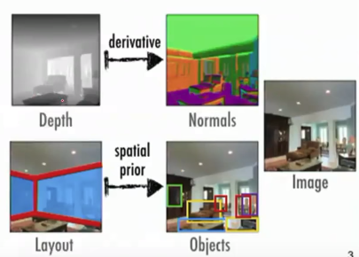
For example, instead you train network for depth and network for normals separately,
you first train network over depth dataset,
and secondly you use transfer learning (with depth-trained network) for normals
Dataset for nomals doesn't need to be labeled because derivative of depth image is normal image
================================================================================
What this project wants to do is supervision-efficiency training with less labeling
================================================================================
Surface normal is to know which direction is a pixel directed to in 3D space?
Computer vision tasks are related
But many of them are unuseful relationships.
And there are also meaningful relationships.
Point is that you can train network in efficient using these relationship.
================================================================================
For example, instead you train network for depth and network for normals separately,
you first train network over depth dataset,
and secondly you use transfer learning (with depth-trained network) for normals
Dataset for nomals doesn't need to be labeled because derivative of depth image is normal image
================================================================================
What this project wants to do is supervision-efficiency training with less labeling
================================================================================
Surface normal is to know which direction is a pixel directed to in 3D space?
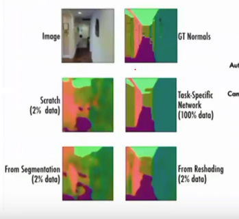 Task-specific network (train over 100% dataset)
Scratch (train over 2% data from 100% dataset)
From segmentation (first train net over segmentation dataset, and use 2% surface normal dataset) bad performance
From reshading (first train net over reshading dataset, and use 2% surface normal dataset) better performance
================================================================================
So, let's perform mapping relationship between tasks into space.
And let's use that relationship in transfer learning.
Task-specific network (train over 100% dataset)
Scratch (train over 2% data from 100% dataset)
From segmentation (first train net over segmentation dataset, and use 2% surface normal dataset) bad performance
From reshading (first train net over reshading dataset, and use 2% surface normal dataset) better performance
================================================================================
So, let's perform mapping relationship between tasks into space.
And let's use that relationship in transfer learning.
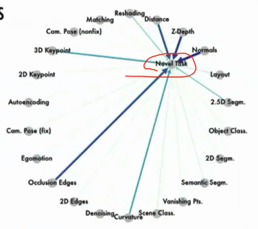 ================================================================================
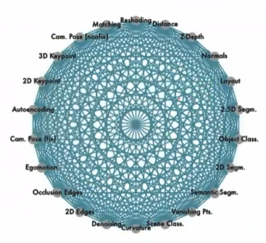
Taskonomy = Task + taxonomy
Taskonomy is a fully computational method for quantifying task relationships.
================================================================================
Taskonomy = Task + taxonomy
Taskonomy is a fully computational method for quantifying task relationships.
 You can see 26 tasks from above illustration.
But it means you can define you own tasks
For example, if you want to solve 50 vision tasks,
you prepare datasets to fit the method represented in this paper.
Then, you can create your own Taskonomy framework.
================================================================================
You can see 26 tasks from above illustration.
But it means you can define you own tasks
For example, if you want to solve 50 vision tasks,
you prepare datasets to fit the method represented in this paper.
Then, you can create your own Taskonomy framework.
================================================================================
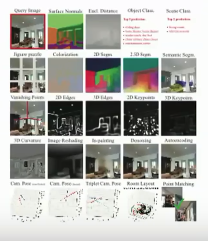
 Final output.
================================================================================
- Tasks which are used for this paper:
26 number of sematic, 2D, 3D tasks
- Each task has labeled dataset
- There are 4 million images in total.
- There are 26 networks which are optimized to each dataset
Final output.
================================================================================
- Tasks which are used for this paper:
26 number of sematic, 2D, 3D tasks
- Each task has labeled dataset
- There are 4 million images in total.
- There are 26 networks which are optimized to each dataset
 ================================================================================
Labeling all images is tedious.
So, authors create "window" which is used for 3D scan.
================================================================================
Tasks
================================================================================
Labeling all images is tedious.
So, authors create "window" which is used for 3D scan.
================================================================================
Tasks
 ================================================================================
2.5D segmentation
2.5D: input has RGB and depth
unsupervised: unlabeled, clustering
================================================================================
================================================================================
2.5D segmentation
2.5D: input has RGB and depth
unsupervised: unlabeled, clustering
================================================================================
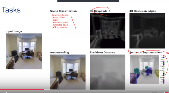 3D keypoints: important points
3D occlusion edges: edge detection which considers occlusion
Euclidean distance:
================================================================================
3D keypoints: important points
3D occlusion edges: edge detection which considers occlusion
Euclidean distance:
================================================================================
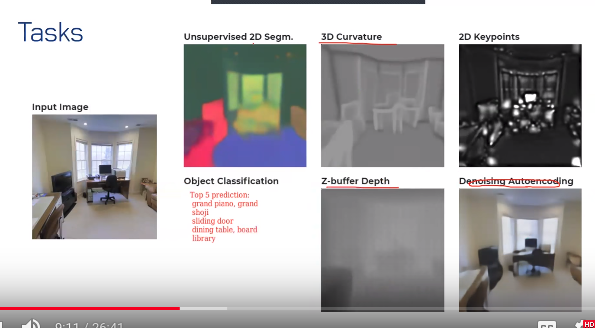 3D curvature: inference bending point
================================================================================
3D curvature: inference bending point
================================================================================
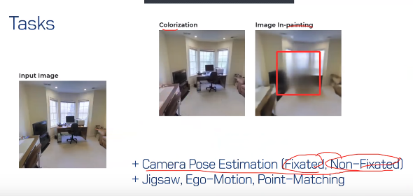 ================================================================================
Ego motion: location of camera in video
================================================================================
================================================================================
Ego motion: location of camera in video
================================================================================
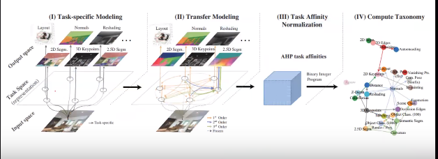 1. You train 26 networks over 26 datasets
2. You perform "transfer modeling" by using 26 pretrained networks.
3. Create task affinity matrix, perform normalization
4. Craete graphs (that is, compute taxonomy)
================================================================================
Task specific modeling
1. You train 26 networks over 26 datasets
2. You perform "transfer modeling" by using 26 pretrained networks.
3. Create task affinity matrix, perform normalization
4. Craete graphs (that is, compute taxonomy)
================================================================================
Task specific modeling
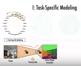 1. Network: encoder + decoder
Unlocked one means it's updated in weights.
2. Detailed network structure.
1. Network: encoder + decoder
Unlocked one means it's updated in weights.
2. Detailed network structure.
 ================================================================================
Transfer modeling
================================================================================
Transfer modeling
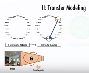 1. Freeze encoder part
2. Add small capacity decoder, and train it over 2% of small dataset.
================================================================================
1. Freeze encoder part
2. Add small capacity decoder, and train it over 2% of small dataset.
================================================================================
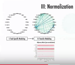 You will get performance after transfer modeling.
You collect all performance values and create matrix with them.
You need to perform normalization because units which are used for 26 tasks are different
For example, some task uses accuracy, some task uses MSE, etc
================================================================================
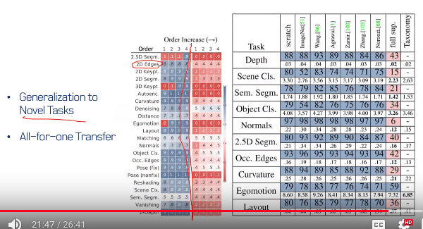
After normalization, you can get following visualized matrix
You will get performance after transfer modeling.
You collect all performance values and create matrix with them.
You need to perform normalization because units which are used for 26 tasks are different
For example, some task uses accuracy, some task uses MSE, etc
================================================================================
After normalization, you can get following visualized matrix
 ================================================================================
Zoomed in view.
================================================================================
Zoomed in view.
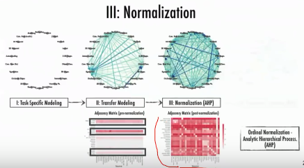
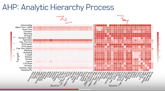 Thicker red in "left table": poorer performance
================================================================================
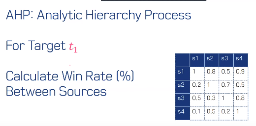
To perform normalization, you can use AHP (analytic hierarchy process)
Thicker red in "left table": poorer performance
================================================================================
To perform normalization, you can use AHP (analytic hierarchy process)
 ================================================================================
Human readable form
================================================================================
Human readable form
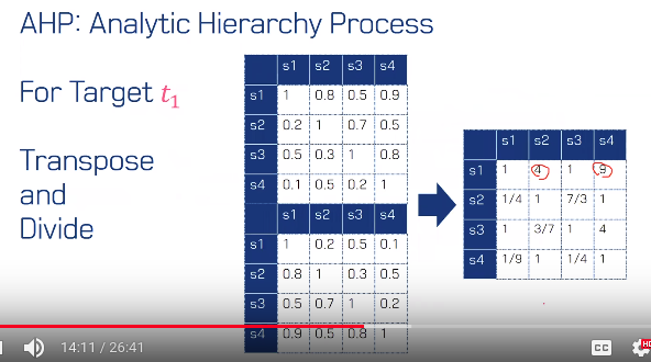 4 means it's 4 times better in relative comparison.
================================================================================
4 means it's 4 times better in relative comparison.
================================================================================
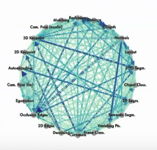
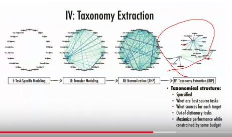 By using above normalized performance data,
you create graph.
================================================================================
When you create graph, you use 3 constraints.
source only: tasks where you can get label easily (you can get 100% task-specific dataset)
target only: tasks where you can't get label easily (you can't get 100% task-specific dataset)
constraint1: only transfer from sources
constraint2: all targets are transferred to
constraint3: not exceed budget (like entire number of image)
================================================================================
By using above normalized performance data,
you create graph.
================================================================================
When you create graph, you use 3 constraints.
source only: tasks where you can get label easily (you can get 100% task-specific dataset)
target only: tasks where you can't get label easily (you can't get 100% task-specific dataset)
constraint1: only transfer from sources
constraint2: all targets are transferred to
constraint3: not exceed budget (like entire number of image)
================================================================================
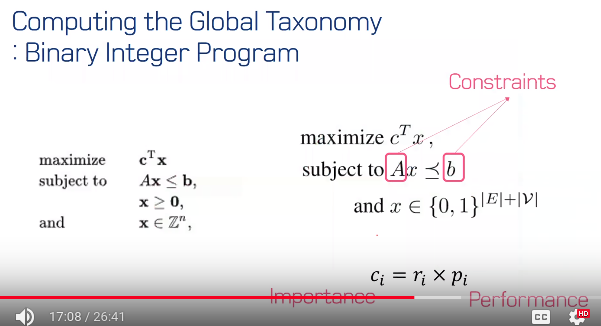 0,1: connect in graph.
E: edge
V: vertices
Target to maximize: $$$c^Tx$$$
$$$c_i=r_i \times p_i$$$
$$$c_i$$$: importance
$$$p_i$$$: performance
$$$r_i$$$: weights between tasks (more/less important tasks)
================================================================================
0,1: connect in graph.
E: edge
V: vertices
Target to maximize: $$$c^Tx$$$
$$$c_i=r_i \times p_i$$$
$$$c_i$$$: importance
$$$p_i$$$: performance
$$$r_i$$$: weights between tasks (more/less important tasks)
================================================================================
 ================================================================================
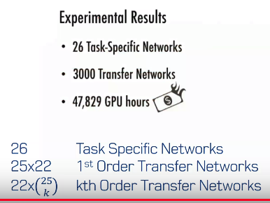 What authors performed
1. they create 26 task specific networks
2. $$$25\times 22$$$ number of 1st order transfer networks
3. 22\times _{25}C_{k} number of kth order transfer networks
3000 transfer networks
47829 GPU hours
================================================================================
What authors performed
1. they create 26 task specific networks
2. $$$25\times 22$$$ number of 1st order transfer networks
3. 22\times _{25}C_{k} number of kth order transfer networks
3000 transfer networks
47829 GPU hours
================================================================================
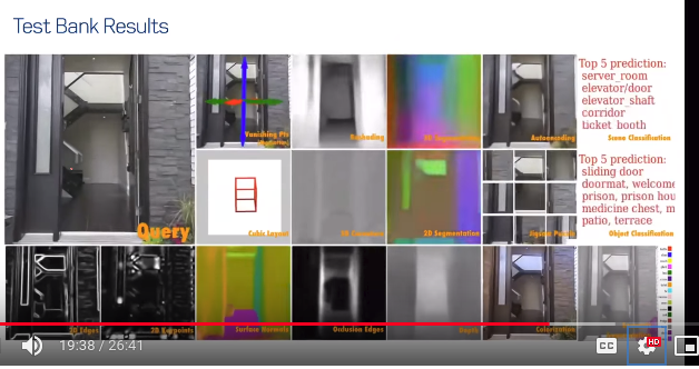 Input query is passed, frame by frame.
================================================================================
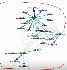
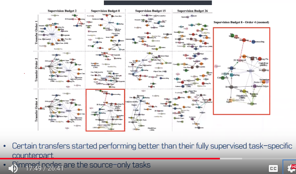
You can do above tasks at the same time after you've create following graphs
Input query is passed, frame by frame.
================================================================================
You can do above tasks at the same time after you've create following graphs
 ================================================================================
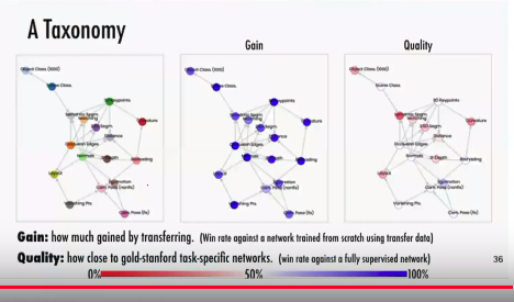 Performance measure: use win rate
Authors define gain and quality
Gain: how is it better than scratch (scratch is what uses 2% data)
Quality: how is it better than what uses 100% data
================================================================================
Performance measure: use win rate
Authors define gain and quality
Gain: how is it better than scratch (scratch is what uses 2% data)
Quality: how is it better than what uses 100% data
================================================================================